A SAS data miner without Enterprise Miner

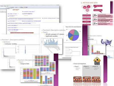
SAS Enterprise Miner (EM) is indeed a fancy tool for a SAS programmer who wants to switch to the field of data mining. It is like the point-and-click camera: you drag several nodes onto the diagram, run it and everything is settled. And I was quite impressed by the resourceful reports and figures automatically generated by SAS EM. Then I spent several months to learn it, passed a SAS certified exam, and finished some pet projects on it. You don’t even need to know anything about statistics to be a data miner. Does that sound too cool to be true?

Some barriers exist for implementing SAS EM in reality. First consideration is the price. SAS charges about 30k for a retail license (I am not sure about the exact price). Only those fat-cat companies, like AT&T, could boast their UNIX-TERADATA-SAS EM complex. Many mid-size or small-size companies can hardly to afford it: they have to do data mining in their own ways with or without SAS. Second is about the installation and maintenance. Since I was taking a training class, I can purchase a license of all SAS products during limited time with a reasonable price. Then I tried numerous times to install SAS EM on my computer and failed. None of my classmates succeeded neither. SAS customer service told me that the standard strategy is to hire a $50k-a-year system engineer, trained by SAS, to install SAS Enterprise Miner properly. Of course, it adds more to the total cost of SAS EM. Third, the running process is contained in a black box. Each time SAS EM would invoke a number of procedures from SAS foundation, but no extra information is available in the log except whether it is a success or failure. For those SAS programmers who tend to check log to find ‘note/warning/error’ message, it is painful experience. I used to run the same process in two computers installed with SAS EM and had distinctive results. Everything was identical, and therefore I could not figure out why I had different results. Fourth, SAS EM is not that efficient. SAS EM applies J2EE to realize the cross-platform feature, which lags the execution time. Data and statistics have to pass through SAS foundation, J2EE until the XML layer of SAS EM. The time to run big data, say more than 100MB data, in a mainstream computer with SAS EM is going to be very long, sometimes intolerable.

Actually, SAS foundation, mainly SAS/BASE and SAS/STAT, is good enough for routine data mining jobs (some procedures may need the license of SAS Enterprise Miner). For example, to emulate the cluster node in SAS EM, we probably have a number of options, such as Proc Cluster, Proc Fastclus, Proc Aceclus, Proc Distance and Proc Tree; to do dimension reduction by PCA or FA, Proc Prinqual, Proc Princomp and Proc Factor are ready to use; to build a decision tree, using Proc Arboretum directly may provide more flexibility. Almost all functionality in SAS EM could be rendered in SAS 9.2. As for the graphics, the SG procedures are handy tools to customize the output images. Macro is a good choice for companies which may need to encapsulate and reuse their codes. If a GUI is desired, Dr. Fernandez in his book suggested using the compiled macros. Besides, we have chance to see what the interim datasets look like.

Still a SAS data miner should be a person who knows statistics. She/he should understand the underlying theory or algorithm; she/he should know how to pick and combine the appropriate procedures corresponding to specific tasks; she/he also should know how to do the dirty work to code and get job done. Overall, the data mining needs to generate not only fun but also meaningful results.


References: George Fernandez. Statistical Data Mining Using SAS Applications, Second Edition (Chapman & Hall/CRC Data Mining and Knowledge Discovery Series). CRC Press.

/*CALL A GUL TO INPUT THE VARIABLES*/
%window mycluster irow=3 rows=33 icolumn=2 columns=60  color=YELLOW
#1    @15 " Cluster Analysis" color=red  attr=underline
#4    @3  "1. Input the SAS Data set name?"  color=blue
#5    @7  "EX: SASHELP.CARS "   attr=rev_video
#6    @7   data 30  required=yes attr=underline
#4    @40  "2. Exploratory graphs ?"  color=blue
#5    @44  " options: YES "      attr=rev_video
#6    @44  explor 20    attr=underline
#7    @3  "3. Input number of cluster   ?"   color=blue
#8    @7   " EX: 5 "    attr=rev_video
#9   @7   num 20    required=yes         attr=underline
#7    @40  "4. Checking for assumptions ?"    color=blue
#8    @44  "options: YES  "  attr=rev_video
#9    @44  assump 10       attr=underline
#10    @3  "5. Input clustering variable(s) ?"   color=blue
#11    @7   "EX: make MSRP "   attr=rev_video
#12    @7   mpred1 80     required=yes           attr=underline
#13    @7   mpred2 80     attr=underline
#13    @90 "contin var" color= blue
#14   @3  "6. Any optional PROC CLUSTER  options?"   color=blue
#15   @7  " EX: method=ave method=cen method=war  k=5 trim=5  "   attr=rev_video
#16   @7  clusopt 80           attr=underline
#17   @3  "7. Input  ID variable ?"      color=blue
#18   @7  " EX: id "       attr=rev_video
#19   @7  ID 30           attr=underline
#17   @40  "8. Variable standardization method ? "     color=blue
#18   @44  prin 30                  attr=underline
#20    @3  "9. Folder to save output?"          color=blue
#21    @7  "EX:  c:\  "        attr=rev_video
#22    @7  output 80              attr=underline
#23    @3 "10. Folder to save graphics ?"    color=blue
#24    @7  "EX: c:\  "       attr=rev_video
#25    @7  dir 80       attr=underline
#29   @3   "11. Display or save SAS graphs?"    color=blue
#30   @7   graph 20      required=yes attr=underline
#33   @10 " USE THE ENTER KEY TO RUN THIS MACRO(don't hit the submit key)  
"color=red attr=rev_video;
%display mycluster;

/*INVOKE THE MACRO USED IN THE GUI*/
libname mylib base "d:\macroproject\cluster";
options sasmstore=mylib mstored;
%mycluster

5D visualiztion: from SAS to Google Motion Chart

Three dimensions are usually regarded as the maximum for data presentation. With the opening of ODS from SAS 9.2 and its graph template language, 3D graphing is no longer a perplexing problem for SAS programmers. However, nowadays magnificent amount of data with multi-dimension structure needs more vivid and simpler way to be displayed.

The emerging of Google Motion Chart now provides a sound solution to visualize data in a more than three dimensions scenario. This web-based analytical technology originated from Dr. Hans Rosling’s innovation. Dr. Rosling and his Gapminder foundation invented a technology to demonstrate the relationship among multiple dimensions by animated bubbles. They developed a lot of bubble plots in Gapminder’s website to discover knowledge form a bulk of public information, especially for regional/national comparison. It soon attracted Google’s attention. In 2008 after an agreement between Dr. Rosling and Google’s two founders, Google launched its Motion Chart gadget. People could create motion chart by using Google Docs, an online alternative to Microsoft’s Office.

The combination between SAS and Google Motion Chart shows a handy and cheap way for up-to-five-dimension data visualization. For Motion Chart, it supports five variables all together in a plot. Commonly the data structure requires time(animation), var1(X axis), var2(Y axis), var3(color) and var4(bubble size). The correlation from var1 to var4 is expected: usually the bubbles with changing color and size tend to move along the diagonal line. Overall 5d visualization can be rendered within such a single plot. In this example, a SAS help dataset ‘SASHELP.SHOES’ is used. The data set has several regions to compare each other. Logged return money is Y-axis, while logged sale money is X-axis. A series of virtual time is given to each region, with inventory as bubble size and the store number as color. By SAS, the data structure in Motion Chart can be prepared quickly. Thus, once the CSV file is uploaded to Google Docs, a motion chart is ready to be published in any webpage. OK, it's time to sit and discover some interesting tendency...

Reference: 1.'Show me--New ways of visualising data’. The Economist. Feb 25th 2010.
2.‘Making data dance’. The Economist. Dec 11st 2010.
3. Google Docs online help center. 2010.

*********(1) Extract data from SASHELP.SHOES***********;
proc sql;
create table test as
select region, Sales, Inventory, Returns, Stores
from sashelp.shoes
order by region , sales desc
;quit;
********(2) Create a random variable for time************;
data test1;
do i=1 by 1 until (last.region);
set test;
by region;
time=today()-i+1;
mytime=put(time, mmddyy8.);
drop i;
output;
end;
run;
********(3) Transform some variables with log**********;
proc sql;
create table test2 as
select region, mytime, log(sales) as logsales, log(returns) as logreturn, Stores as storenum, Inventory
from test1
order by region, mytime
;quit;
********(4) Export data as CSV***************;
proc export data=test2 outfile='C:\Users\Yanyi\Desktop\test.csv' replace;
run;
*******(5) Upload CSV to Google Docs************;
******(6)  Create Google Motion Chart manually**********;

**********END*********TEST PASSED 12DEC2010****************************;

Proc Fcmp(3): brute force for a distribution's pdf

Proc Fcmp can produce arbitrary distribution formulas. In this example, suppose that I don’t know too much statistics, what if I want to evaluate the pdf of the absolute value of the subtraction between two independent random variable from the uniform distributions? In this example, probably we can follow such procedures: (1) use Proc Kde to find the kernel distribution and make a guess about what this distribution is; (2) use Proc Fcmp to make the pdf of the distribution; (3) use Proc Model to fit the test dataset and find the parameters; (4) use the simulation to validate the hypothesis. Thus, such a method may be a useable solution to evaluate distribution of a random variable, if without stringent mathematical proof.

*************(1) The distribution of the absolute value of between two uniform distribution*****;
data distance;
do i=1 to 10000;
x1=ranuni(0);
x2=ranuni(0);
x=abs(x1-x2);
drop i;
output;
end;
run;
proc sgplot;
histogram x1/transparency=0.3;
histogram x2/transparency=0.7;
histogram x/transparency=0.8;
run;

************(2) Observe the kernel distribution ************;
ods graphics on;
proc kde data=distance;
univar x /plots=all out=myden;
run;
ods graphics off;

***********(3) Fit with Beta distribution*****************;
proc fcmp outlib = sasuser.myfunc.math;
function betadist(a,b,x);
density=(beta(a,b))**(-1)*x**(a-1)*(1-x)**(b-1);
return(density);
endsub;
run;

options cmplib = sasuser.myfunc nodate ls=80;
proc model data=myden(rename=(value=x));
density=betadist(a,b,x);
fit density;
quit;

************(4) Look at the distribution again***************;
data newdata;
do i=1 to 1E5;
y=rand('beta', 1, 2);
output;
end;
run;

proc sgplot data=newdata;
histogram y/fillattrs=(color=green) ;
run;
********************END********************;

Proc Fcmp(2): a subroutine for Binomial-CRR model

Problems: Quote for six-month American style euro currency options on plain vanilla, Max[S-K,0]and 〖Max[S-K,0]〗^0.5. Exchange rate S_0=$1.3721 /euro
Six-month continuously compounded inter-bank rates: r=0.4472%,r_f=1.2840%.
Assumptions:The exchange rate for euro follows an iid log normal price changes and volatility is constant.
Methodology:Binomial Model is used to price American currency options on euros.
We calculate the payoffs at time T and discount payoffs to the prior time step. Under the risk neutral probability measure,
c_(t-1)=(q×c_u+(1-q)×c_d)/R
Since these two options are American styles, we need to check for optimal early exercise at each node of the binomial tree. For these two currency options, we check Max[S-K,c_(t-1),0] and Max[〖Max[S-K,0]〗^0.5,c_(t-1) ] . Matlab is the software used to implement the binomial model.
--Parameters:1. Time steps n
As the number of time steps n increases, we can apply CRR model and the binomial model approaches real world price changes. We choose n=80,h=T/n=0.5/80=0.00625.
2. u and dWe choose CRR model to define u and d for binomial model.
u=e^(σ√h) ; d=1/u=e^(-σ√h)
Where h is the length of the binomial times step and σ is the annualized log price change volatility.
3. Annualized log price change volatility σThe daily log changes and daily squared log changes for two year exchange rates from 11/5/2008 – 11/5/2010 are as follows. We consider the volatility to be constant since 05/01/2009. Thus, we choose the historical prices from 05/01/2009-11/5/2010 and apply the volatility of the daily log changes as an estimate. Then the annualized log price change volatility equals the square root of the trading days in one year (252 days) times the daily log price change volatility.
σ=√252×σ_daily
4. Risk Neutral Measure QOptions on currencies can be regarded as an asset providing a yield at the foreign risk-free rate of interest. Thus, the risk neutral probability measure Q :
q=(e^((r-r_f ) )-d)/(u-d) ;
1-q= 〖u- e〗^((r-r_f ) )/(u-d)
5. Strike Price KSet strike price K from $1.3000/euro to $1.5000/euro with $0.005 per euro increments.
Reference: 1. John C. Hull.Options, Futures and Other Derivatives, 7th edition. Prentice Hall. 2008.
2. Base SAS 9.2 Procedures Guide. SAS Publishing. 2009

**********************AUTHOR(DAPANGMAO)----HCHAO8@GMAIL.COM***********************************;
****************(1) CONSTRUCT € TO $ EXCHANGE RATIO VECTOR******************;
data vector;
attrib value informat=dollar10.4 format=dollar10.4 ;
StrikeS=1.3000;  
StrikeE=1.5000;
Increment=0.005;
do value=StrikeS to StrikeE by  Increment;
drop StrikeS StrikeE Increment;
output;
end;
run;

**************(2) BUILD THE FUNCTION TO EVALUATE OPTION PRICES********;
proc fcmp outlib = myfunc.finance.subrout;
subroutine mysubr(T, n, r, rf, s0, sigma, c1[*], c2[*]);
/*Two vectors are output arguments*/
outargs c1, c2;
/*Inside calculation from input arguments*/
dt=T/n;
length=dim(c1);
u=exp(sigma*sqrt(dt));
d=1/u;
q=(exp((r-rf)*dt)-d)/(u-d);
/*Announce 4 arrays -- 1 vector and 3 matrixes */
array k[1]/ nosymbols;
array s[1] /nosymbols;
array x1[1] /nosymbols;
array x2[1] /nosymbols;
n=n+1;
/*The sizes of the arrays are specified*/
call dynamic_array(s, n, n);
call dynamic_array(x1, n, n);
call dynamic_array(x2, n, n);
call dynamic_array(k, length);
/*Read the exchange ratio into function*/
rc=read_array('vector', k);
/*Assign values to S matrix */
call zeromatrix(s);
S[1,1]=S0;
do _col=2 to n ;
do _row=1 to n;
S[_row,_col]=S0*u**(_col-_row)*d**(_row-1);
if _row gt _col then S[_row, _col]=0;
end;
end;
/*Generate final option vectors */
do i=1 to length;
x=k[i];
call zeromatrix (x1);
call zeromatrix (x2);
do j=1 to n;
x1[j,n]=max(S[j,n]-x,0);   
x2[j,n]=max(S[j,n]-x,0)**0.5;     
end;
do _col=(n-1) to 1 by -1;
do _row=1 to (n-1) by 1;
h=exp(-r*dt)*(q*x1[_row,_col+1]+(1-q)*x1[_row+1,_col+1]);
h2=exp(-r*dt)*(q*x2[_row,_col+1]+(1-q)*x2[_row+1,_col+1]);
x1[_row,_col]=max(S[_row,_col]-X,h,0);    
x2[_row,_col]=max( max(S[_row,_col]-x ,0) **0.5, h2);  
end;           
c1[i]=x1[1,1];
c2[i]=x2[1,1];
end;
end;
endsub;
run;
quit;

***********SOME INITIAL VALUES*****************;
/*T=1/2;*/
/*n=80;*/
/*r=0.004472;    */
/*rf=0.01284;*/
/*S0=1.3721;*/
/*Sigma=0.1074*/

**************(3) MEASURE THE LENGTH OF PRICING VECTOR**************;
proc sql;
select count(*) into: vecnum from vector;
quit;

**************(4) USE THE SUBROUTINE TO GENERATE TWO VECTORS********************;
options cmplib = (myfunc.finance);
data final;
array c1[&vecnum] _temporary_;
array c2[&vecnum] _temporary_;
call mysubr(0.5, 80, 0.004472, 0.01284, 1.3721, 0.1074, c1, c2);   /*subroutine mysubr(T, n, r, rf, s0, sigma, c1[*], c2[*]);*/
do i=1 to dim(c1);
c1value= c1[i];
c2value=c2[i];
output;
end;
run;
****************TEST PASSED ----------- END****************************;

Find the 'right' SAS functions

How many functions SAS has? Well, it sounds like a job interview question. For SAS 9.2, by querying the system dictionary (sashelp.vfunc or dictionary.functions), the exact answer is 946, including all functions and call routines. There are two types - unicode/bit based on input argument, while three types –numeric/character/bitwise based on output argument. Again according to their usage[1], the common SAS functionscan be categorized into several types: array(3), bitwise logical operation(3), PERL regular expression(11), character(91), time(38), descriptive statistics(32), random number(22), probability(18) , mathematics(36), finance(32), etc.

Some functions have evolved for several generations Since SAS has development history of more than 40 years. For example, there are 6 functions from SAS dictionary for random number generator from normal distribution, including ‘normal’, ‘rannor’ and its call routine, ‘rannorm’ and its call routine, and ‘rand’. All functions need seeds to produce random numbers and the random number queue can be replicated if with the same seed. The difference is that the latest one ‘rand’ has astronomical possibilities of seeds, while the older types only contains merely 2 trillion seeds that can cause dependence among various random number queues.

SAS handles data with rows as units (SAS calls row as observation), which is a unique characteristics, while most other software packages tend to process data with columns or vectors. Thus, many summarization functions in Data step only work on the ‘right’ by combining all variables in a row. As for vertical summarization, the SAS procedures are more appropriate, such as Proc Summary, Proc Means or Proc report. In a word, if we prefer SAS Data step, a transposition may be necessary.

Reference: 1. SAS 9.2 Language Reference: Dictionary, Third Edition. SAS Publishing. 2009.
2. Ron Cody. SAS Functions by Example, Second Edition. 2010.

/**********************AUTHOR(DAPANGMAO)----HCHAO8@GMAIL.COM***********************************;
*(1)CALCULATE THE COMPOSITION OF SAS FUNCTIONS*/
proc sgplot data=sashelp.vfunc;
vbar fnctype/barwidth=0.5
transparency=0.2 ; 
run;

proc sgplot data=sashelp.vfunc;
vbar source;
run;
proc sgplot data=sashelp.vfunc;
scatter x= source y=fnctype;
run;
proc sql;
select *
from sashelp.vfunc
where lowcase(fncname) in ('rannorm', 'rannor', 'normal', 'rand');
quit;
proc freq data=sashelp.vfunc;
tables fnctype*source/nopercent nocum norow nocol;
run;

/*(2)COMPARE SERVAL RANDOM FUNCTIONS*/
data one;
call streaminit(1234);
do i=1 to 10000;
x1=rannorm(1234);
x2=rannor(1234);
x3=normal(1234);
x4=rand('normal');
output;
end;
run;
data two;
seed1 = 1;
seed2 = 3;
seed3 = 5;
seed4=7;
do i = 1 to 10000;
call rannor(seed1, x1);
call rannor(seed2, x2);
call rannor(seed3, x3);
call rannor(seed4, x4);
output;
end;
run;
%macro test(input);
proc sgscatter data = &input;
title 'Independence test';
plot x1*x2 x1*x3 x3*x2 x1*x4 x2*x4 x3*x4 / markerattrs = (size = 1);
run;
%mend test;

/*(3)PICK OUT THE LARGEST THREE FROM VARIOUS TRANSACTIONS*/
data test;
attrib amt informat=dollar10.2 format=dollar10.2;
do id=1 to 10;
times=ceil(100*ranuni(12345));
do i=1 to times;
amt=10000*ranuni(123);
output;
end;
end;
drop i times;
run;
proc sort data=test out=test1; 
by id descending amt;
run;
data test2;
do _n_=1 by 1 until(last.id);
set test1 ;
by id;
if _n_<4 then output;
end;
run;
proc transpose data=test out=test3(drop=_name_);
by id notsorted;
var amt;
run;
proc sql;
select name into: vname separated by ', '
from sashelp.vcolumn
where libname='WORK'
and memname='TEST3'
and name contains 'COL'
;quit;
%put &vname;
data test4;
set test3;
call sortn(of &vname);  
vstd=std(of &vname);
vmax=max(of &vname);
vmean=mean(of &vname);
vmedian=median(of &vname);
vrange=range(of &vname);
vnum=n(of &vname);
vmissing=nmiss(of &vname);
no1=largest(1, of &vname);
no2=largest(2, of &vname);
no3=largest(3, of &vname);
run;

Why I like Mainframe SAS

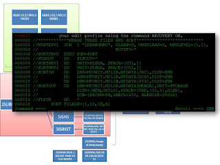
I was horrified by Mainframe SAS first time when I saw it. I struggled many times to let SAS output ‘Hello World’ to the log and failed, and then I started to sweat. Finally my colleague came to rescue me by teaching me to how to insert JCL before the SAS codes. In a world where every programmer is spoiled by shinning GUI or IDE, I felt fairly uncomfortable to code flashing characters in a floating window by ISPF, a seemly unfriendly text editor. To make things even worse, SAS’s interactive mode was forbidden in my team. Then to test a program is like fumbling for the end in a dark tunnel: you don’t know what your result will be like until the system told you it is ready after minutes’ waiting. As the result, I just found myself totally lost. Eventually I survived in the mainframe kingdom and now I start to like MF SAS. Even though it is a relic from ancient ‘punch-card’ time, MF SAS still has some unique strength, comparing with its more popular peers, such as UNIX SAS and PC SAS.

The power of MF SAS comes from its combination with z/OS, ISPF and JCL as a whole. (1) Nature of sharing. Since we are dealing with a distant server through 3270 terminal, all datasets and program codes can be easily shared. Thus, it is not necessary to set up any FTP or file sharing server. Thousands of coworkers can seamlessly share their progress and keep synchronized. (2) Native sorting and concatenation. JCL can concatenate multiple files together simply by naming them in Data Definition step. System-wise Sort program is also very handy. (3) Quick setup of system options. JCL can help SAS specify some system options, which cannot be switched on/off within SAS itself. For example, the SASLIST and SASLOG files can be outputted to somewhere we want to check later. (4) Scheduling of a job. The code in JES, part of JCL, can order SAS to run at certain time without human’s intervention. That is a really cool feature: how about that SAS starts to run from 2am and I check the overnight result in the morning. (5) Pipeline statement in DD. From SAS 9.1, SAS supports pipeline, by which a library in MF can be translated into an equivalent library in SAS. It will save time to define datasets. (6) Subroutines in calling ISPF commands. SAS provides some subroutines, such as CALL ISPEXEC and CALL ISPLINK, to integrate ISPF. Besides those advantages above, another good thing is that in ISPF the datasets can be manually modified. That is a blessing for people tends to change small mistakes by themselves, instead of running program once again. In conclusion, SAS thrived from the mainframe period, and MF SAS is still visible and alive. Let us enjoy it and hope it to flourish again.

Reference:1. SAS®9.1.3 Companion for z/OS. SAS Publishing. 2004
2. Introduction to the New Mainframe: z/OS Basics. IBM Press. 2009

**********************AUTHOR(DAPANGMAO)----HCHAO8@GMAIL.COM***********************************;
//************MERGE THREE FILES AND SORT**************************
//MYSTEP01  JOB  1 'DAPANGMAO', CLASS=C, MSGCLASS=X, MSGLEVEL=(1,1),
//                              NOTIFY=*
//          EXEC PGM=SORT
//SORTIN    DD   DSN=MYUNIT.MYLIB.MYDATA(CAT),DISP=SHR
//          DD   DSN=MYUNIT.MYLIB.MYDATA(DOG),DISP=SHR
//          DD   DSN=MYUNIT.MYLIB.MYDATA(PIG),DISP=SHR
//SORTOUT   DD   DSN=MYUNIT.MYLIB.MYDATA(MERGE),UNIT=STORAGE
//               DISP=(NEW,CATLG),SPACE=(TRK,(25,5),RLSE),
//               DCB=(RECFM=FB,LRECL=250, BLKSIZE=25000)
//SYSOUT    DD   SYSOUT=*
//SYSIN     DD   *
SORT FILEDS=(1,10,CH,A)
/*
//*******************SAS PROCEDURE TO CALCULATE MEANS*************
//MYSTEP02  JOB 1 'DAPANGMAO', CLASS=C, MSGCLASS=X,MSGCLEVEL=(1,1)
//                              NOTIFY=*
//*MAIN DEADLINE=(0400,A,12152010)
//          EXEC SAS,
//               OPTIONS='LOG=OUTLOG PRINT=OUTPRINT'
//*ALTERNAT EXEC SAS, CONFIG= MYUNIT.MYLIB.MYCONFIG
//MYINPUT   DD   DSN=&&MERGE,DISP=SHR
//OUTLOG    DD   DSN=MYUNIT.MYLIB.LOGDATA.OUTLOG,DISP=OLD
//OUTPRINT  DD   DSN=MYUNIT.MYLIB.LOGDATA.OUTPRINT,DISP=OLD

DATA MERGE1;
INFILE MYINPUT;
INPUT ANIMAL &9.  TYPE &5. NUMBER 5.;
RUN;

PROC MEANS DATA=MERGE1;
CLASS TYPE;
VAR NUMBER;
RUN;
/*
//*******************BUILD A PIPE LIBRARY FOR SAS*************
//MYSTEP03  JOB  1 'DAPANGMAO', CLASS=C, MSGCLASS=X, MASGLEVEL=(1,1),
//                   NOTIFY=*
//          EXEC SAS
//PIPELIB   DD   DSN=MYUNIT.MYLIB.MYDATA,LRECL=6144,RECFM=F,DSORG=PS,
//               SUBSYS=(BP01,CLOSESYNC,ERC=DUMMY),LABEL=(,,,OUT)
//ADDON     DD   DSN=MYUNIT.MYLIB.MYDATA(FOX),DISP=SHR

DATA PIPELIB.CAT;
INFILE ADDON;
OUTPUT;
RUN;

DATA _NULL_;
CALL ISPEXEC(’SELECT PANEL(MAINDEV)’);
IF PLIRETV = 0 THEN PUT PLIRETV=;
RUN;
/*                         

The efficiency of five SAS methods in multi-dataset merging

Introduction: Merging two or multiple datasets is essential for many ‘data people’. Yes, it is a dirty and routine job. Everyone wants to get it done quick and accurate. Actually, SAS has many ways to tackle this job[3]. In two competing papers from SAS Global Conference 2009, Qinfeng Liang[1] described five ways to marge a base table and a lookup table regarding the healthcare industry, while David Franklin[2] pictured eight methods to combine patient and effect datasets in a typical pharmaceutical scenario. Here I would like to extend the discussion further: one base table and two lookup tables. I would like to see which one of the solutions would cost less hardware resource and, most importantly, system time.

Method: The base table was generated with 10 million sequential numbers. Two subset tables were randomly chosen from the base table and kept unsorted until a method was applied, and each contains 1 million records. Five methods, Proc SQL, Data step Merge, Proc Format, Data step Hash object and Data step key-set were utilized and compared. System time was summed for each method. The requirement for memory was recorded.

Result: As expected, methods related to data step consume less memory. Key-data structure methods, including Proc SQL, Proc Format and Data step Hash object, ask much more memory. However, in-memory processing does not deliver much help to the time. Proc Format and Data step Hash object still spend above-average time, while obviously Data step set-key costs most time in waiting.

Discussion: Amazingly, even as an ancient technology (maybe 40 years old), Data step Merge is the winner in this competition with both satisfied time and least memory usage. It is also code-efficient. Proc SQL is the second choice. Hash object doesn’t show its edge as other authors suggested. Proc format and Data step key-set are the least favored ones. I also tried Data step Array, and I found that it was very difficult to load the lookup table and eventually I gave up the attempts. The solution by Proc Format is hard to code for multiple table joining, since each has to build an individual format and Proc Format has no batch mode. In conclusion, the choice of the best method depends on specific needs or situation. Old methods, like Data step Merge, can still perform as well as others do, sometimes even better.

References: 1. Qingfeng Liang. Choosing the Right Technique to Merge Large Data Sets Efficiently. SAS Global Forum 2009
2. David Franklin. Merging Data Eight Different Ways. SAS Global Forum 2009
3. SAS® Certification Prep Guide: Advanced Programming for SAS®9. SAS Institute Inc. 2007

********************GENERATE THREE TABLES TO JOIN BY SIMULATION****************;
********************1. GENERATE THE BASE TABLE;
data base;
do number=1 to 1E7;
output;
end;
run;

********************2. GENERATE THE SUB TABLE TO BE JOINED;
proc sql outobs=1000000;
create table sub1 as
select number 
from base 
order by ranuni(43234);
create table sub2 as
select number 
from base 
order by ranuni(45954);
quit;
********************END OF SIMULATION ****************;


*******************MERGE STEPS******************;
*******************1. PROC SQL;
proc sql;
create table sqlmerge as
select a.number, b.number as var1, c.number as var2
from base as a left join sub1 as b on a.number = b.number
left join sub2 as c on  a.number=c.number;
quit;

*******************2. DATA STEP MERGE;
proc sort data=sub1 out=sub1_s;
by number;
run;
proc sort data=sub2 out=sub2_s;
by number;
run;
data datastepmerge;
merge base(in=a) sub1_s(in=b) sub2_s(in=c);
by number;
if b then var1=number;
if c then var2=number;
if a;
run;
/*ALTERNATIVE 1 --  USE DATA SET INDEX TO APPLY DATA STEP MERGE*/
/*
proc sql;
create index number on base;
create index number on sub1;
create index number on sub2;
quit;
data datastepmerge;
merge base(in=a) sub1(in=b) sub2(in=c);
by number;
if b then var1=number;
if c then var2=number;
if a;
run;
*/
/*ALTERNATIVE 2 --  USE DATA SET VIEW TO APPLY DATA STEP MERGE*/
/*
proc sql;
create view  Vbase as select * from base order by number ;
create view  Vsub1 as select * from sub1 order by number;
create view  Vsub2 as select * from sub2 order by number;
quit;
data datastepmerge;
merge Vbase(in=a) Vsub1(in=b) Vsub2(in=c);
by number;
if b then var1=number;
if c then var2=number;
if a;
run;
*/

*******************3. PROC FORMAT;
data sub1_fmt;
length start $12; 
retain fmtname "sub1_fmt";
set sub1 end=lastobs;
do _n_=1 until (lastobs);
start=input(number, $12.);
label=start;
drop number;
output;
end;
if lastobs then do;
start ='other' ;
label= '.';
output;
end;
run;
proc format cntlin=sub1_fmt;
run;

data sub2_fmt;
length start $12; 
retain fmtname "sub2_fmt";
set sub2 end=lastobs;
do _n_=1 until (lastobs);
start=input(number, $12.);
label=start;
drop number;
output;
end;
if lastobs then do;
start ='other' ;
label= '.';
output;
end;
run;
proc format cntlin=sub2_fmt;
run;

data formatmerge;
set base;
var1=put(number, sub1_fmt.);
var2=put(number, sub2_fmt.);
run;

*******************4. DATA STEP HASH OBJECT;
data hashobjmerge;
if _n_=1 then do;
declare hash sub1_h(dataset: 'sub1');
sub1_h.defineKey('number');
sub1_h.defineDone();
declare hash sub2_h(dataset: 'sub2');
sub2_h.defineKey('number');
sub2_h.defineDone();
end;
set base;
var1=number; 
var2=number;
if sub1_h.find() then call missing(var1); 
if sub2_h.find() then call missing(var2);
run;

**********5. DATA STEP KEY-SET;
proc sql;
create table sub1_ix as
select *, number as var1
from sub1;
create index number on sub1_ix;
quit;
data sub2_ix(index=(number /unique /nomiss));
set sub2;
var2=number;
run;
data keysetmerge;
set base;
set sub1_ix KEY=number /unique;
if _IORC_ then do;
_ERROR_=0;
var1='';
end;
set sub2_ix key=number/unique;
if _IORC_ then do;
_ERROR_=0;
var2='';
end;
run;
quit;
*******************END OF COMPARISION************;

Proc Fcmp(1): from VBA to SAS

Why use SAS in finance: SAS is a distinguished software package in statistics with more than 40-year development history. Starting from as a scripting tool to do ANOVA for agricultural experimental design in North Carolina, SAS has been heavily built on generalized linear model. For example, SAS institute consistently improve linear model procedures, from Proc Anova, Proc Glm, Proc Mixed to the latest Proc Glimmix. In a summary, SAS is pretty good at processing and analyzing any linear or non-linear models. However, the foundation for finance model, such as fixed income products and derivatives, is continuous-time equations, such as Black-Scholes formula. Most likely, quantitative analysts tend to price the products by solving those equations. So, in a word, the finance analyst is always working with equations, or many equations. Obviously here SAS is not good at it. Yes, SAS has more than 900 functions. And they are still not enough to keep up with the fast-pace of Wall Street. That is why the quants use Matlab, C++ and Excel VBA, instead of SAS. Then how the quants need to create their own equations in SAS? And how they build their function library or include the 3rd party library? Proc Fcmp may be the rescue.
Why Proc Fcmp? Finally we have Proc Fcmp, an equation editor. Proc Fcmp is a formidable tool for building function and even function library. All self-built or third party functions are stored in customer-specified package for future usage. Like Excel VBA, Proc Fcmp can construct equivalent subroutine and function. The nice thing is that all the function-based variables are encapsulated without any explicit declaration ( I hate nested macros: the variables would surf around from here to there). In addition, SAS Function Editor is an excellent tool viewer to manage and check all functions.
Conclusion: Look at the codes below, you see that Excel VBA and SAS Proc Fcmp are quite similar. A VBA developer can switch to SAS developer very smoothly in a short period. Also many people can work with a function package simultaneously through a distant SAS server, while each of them builds individual function. The quants may feel more comfortable to use SAS than VBA. Another good thing is that, by using Proc Proto, C++ function can be introduced into Proc Fcmp. That means that even C++ developer can also explore the turf of SAS language. Given that SAS is also a wonderful database management software, I expect that more and more people would embrace SAS through Proc Fcmp in the finance area.

Reference: Jørgen Boysen Hansen. Using the new features of Proc Fcmp in risk management at dong energy A/S. DONG Energy A/S.

'USE EXCEL VBA TO TO GRADE THE SCORES OF 28 STUDENTS
Function Grade(score)
If IsGrade(score) Then
Select Case score
Case Is <= 60  Grade = "F"             
Case 60.5 To 70   Grade = "D"            
Case 70.5 To 80   Grade = "C"            
Case 80.5 To 90   Grade = "B"             
Case IS > 90      Grade = "A"
End Select
Else
Grade = " "
End If
End Function

/*USE PROC FCMP TO GENERATE THE FUNCTION */
proc fcmp outlib=sasuser.myfunction.grade;
function grade(score);
select;
when (Score GE 90) return ("A");
when (Score GE 80) return ("B");
when(Score GE 70) return ("C");
when (Score GE 60) return ("D");
when (Score NE .)   return ("F");
otherwise;
end;
endsub;
run;
quit;
/*APPLY THE FUNCTION TO GRADE THE SCORES OF 28 STUDENTS*/
options cmplib=sasuser.myfunction;
data exam_one_graded;
set exam_one;
Grade_one=grade(score);
run;

Proc Arboretum: a secret weapon in decision tree

Introduction: Decision tree, such as CHAID and CART, is a power predicative tool in statistical learning and business intelligence. Starting from SAS®9.1, the ARBORETUM procedure provided facilities to interactively build and deploy decision tress. Even though it is still an experiment procedure, the ARBORETUM procedure has comprehensive features for classification and predication. And the ARBORETUM procedure is also the foundation of decision tree node in SAS Enterprise Miner.
Method: A common SAS dataset ’sashelp.cars’ was divided into three parts of equal size: training, validation and scoring. Two methods were applied: the target variable ‘origin’ as nominal level and the target variable ’ MSRP’ as interval level.
Result: the codes below introduced how to use PROC RBORETUM to train, validate and score datasets based on decision tree. The generated DATA step codes were stored in two flat text files.
Conclusion: the ARBORETUM procedure is quick and versatile for applying decision tree for any size of dataset. It is really a secret weapon in the procedure stockpile of SAS.

Reference: Xiangxiang Meng. Using the SGSCATTER Procedure to Create High-Quality Scatter Plots. SAS Global Forum 2010.

/*DIVIDE THE ORIGINAL DATA INTO 3 PARTS: 1:1:1*/
data cars;
set sashelp.cars;
_index=_n_;
run;
proc sort data=cars;by origin;run;
proc surveyselect data=cars samprate=0.3333  out=train;
strata origin /alloc=prop  ;
run;
proc sql;
create table cars2 as
select  * from cars
where _index not in ( select _index from train)
;quit;
proc surveyselect data=cars2 samprate=0.5  out=validation;
strata origin /alloc=prop  ;
run;
proc sql;
create table test as
select  * from cars2
where _index not in ( select _index from validation)
;quit;
proc datasets;
delete cars2 cars;
run;

/*TARGET VARIABLE: NOMINAL*/
filename code_1 'C:\code_1.txt';
proc arboretum data=train;
target origin / level=nominal;
input MSRP Cylinders Length  Wheelbase MPG_City MPG_Highway Invoice Weight Horsepower/ level=interval;
input EngineSize/level=ordinal;
input  DriveTrain Type /level=nominal;
assess validata=validation;
code file=code_1;
score data=test out=scorecard outfit=scorefit;
save   IMPORTANCE=imp1 MODEL=mymodel  NODESTATS=nodstat1  RULES=rul1 SEQUENCE=seq1 SIM=sim1  STATSBYNODE= statb1 SUM=sum1
;
run;
quit;

/*TARGET VARIABLE: INTERVAL*/
filename code_2 'C:\code_2.txt';
proc arboretum data=train;
target MSRP / level=interval;
input  Cylinders Length  Wheelbase MPG_City MPG_Highway Weight Horsepower/ level=interval;
input EngineSize/level=ordinal;
input  DriveTrain Type origin /level=nominal;
assess validata=validation;
code file=code_2;
score data=test out=scorecard2 outfit=scorefit2;
save   IMPORTANCE=imp2 MODEL=mymode2  NODESTATS=nodstat2  RULES=rul2 SEQUENCE=seq2 SIM=sim2  STATSBYNODE= statb2 SUM=sum2
;
run;
quit;

Multi-study research on Bovine respiratory disease

Situation:The purpose of this research was to (1) to explore a recent multi-study approach (Arends, et al. 2008) in combining observational survival data instead of traditional meta-analysis, and (2) to develop multivariate random-effects models with or without covariates to aggregate three studies on Bovine Respiratory Disease (BRD). Models were constructed, assessed and presented by programming in SAS®.
Task:The multivariate random-effects models built in this report demonstrated improved efficiency, and generalizability and precision.
Action:First the modeling is simple and easy to explain. Second the aggregation of the three studies was accomplished and survival proportion with CIs were updated. Second the estimated survival proportions by such models, showing reduced standard error, are more precise than Kaplan-Meier estimated survival proportion or Cox proportion hazards regression estimated survival proportion.
Result:Transformed data with LOCF by LAST. and FIRST. variables;Proposed a multi-survival-data model by PROC PHREG/LIFETEST/GLIMMIX and increased >70% precision; Rendered graphs by PROC SGPLOT/SGPANEL and SAS Graph Template language; Generated table and listing by PROC REPORT/SQL/TABULATE

Reference: Arends LR, Hunink MG, Stijnen T. Meta-analysis of summary survival curve data. Stat Med. 2008 Sep 30;27(22):4381-96.
Code I

/******************************************************************/
PROGRAM: NO-COVARIATES MODEL
PURPOSE: CREATE ARENDS' MODEL FOR DATA SETS 1 & 2 $ 3 BY NO-COVARIATE METHOD
AUTHOR: ---------------
LAST REVISE DATE:  JUNE 18, 2010
LAST TEST DATE: JUNE 18, 2010
*****************************************************************/
libname source 'd:\animal_data'; /*set up the library for the input*/;
/*set up the work library for output*/;

********************BEGINNING OF THE PROGRAM********************;

**********#1 USE PROC LIFETEST**********;
ods graphics on;
proc lifetest data = source.data_1_2_3 OUTSURV =pred_bylifetest  plots=(ls,lls) alpha=0.05;   /*generate the log and loglog transformation plots*/
title 'Figure 2A & 2B ';
time DOF_FIRST_TX * status(0);
strata source;
run;
ods graphics off;
**********END**********;

**********#2 GENERATE SURVIVAL CURVE BY WEEKS**********;
proc sgplot data=pred_bylifetest;
title 'Figure 1';
step x= DOF_FIRST_TX y=survival /group=source;
yaxis min=0;
xaxis grid values=(0, 7, 14, 21, 28, 35, 42, 49, 56);
run;
**********END**********;

**********#3 MANIPULATION OF THE PREDICTED DATA SET BY PROC LIFETEST**********;
data pred_bylifetest;
set pred_bylifetest;
*****CLEAN THE DATA SET;
if survival=.  then delete;                 /*delete invalid information for survival proportion*/
*****ADD TWO VARIABLES;
if survival ne 1 then  lls=log(-log(survival));                      /*add the log(-log()) transformed survival proportion*/
if DOF_FIRST_TX gt 0 then ln_day=log(DOF_FIRST_TX);                                 /*add the log transformed time*/
*****ADD LABELS;
label DOF_FIRST_TX='Days to the first treatment'                    
ln_day='log(Days to the first treatment)'
lls='log(-log(Survival probability function))';
run;
**********END**********;

**********#4 FIT THE SCATTER DOTS WITH LEAST-SQUAR LINES**********;
*****FIT THE SCATTER DOTS WITH SEPARATE STRAIGHT LINES;
proc sgplot data=pred_bylifetest;
title 'Figure 2C';
scatter x=ln_day y=lls/group=source;
reg  x=ln_day y=lls/group=source degree=1;        /*fit the scatter dots with the straight lines separately*/
yaxis label='log(-log(Survival probability))';
xaxis label='log(Days to the first treatment)';
run;
*****FIT THE SCATTER DOTS WITH SEPARATE QUARRATIC CURVES;
proc sgplot data=pred_bylifetest;
title 'Figure 2D';
scatter x=ln_day y=lls/group=source;   
reg  x=ln_day y=lls/group=source degree=2;          /*fit the scatter dots with the quadratic curves separately*/
yaxis label='log(-log(Survival probability))';
xaxis label='log(Days to the first treatment)';
run;
**********END**********;

**********#5 USE PROC MIXED TO GENERATE COEFFICIENTS**********;
*****GENERATE THE COEFFICIENTS WITH THE LINEAR MODEL;
proc mixed data= pred_bylifetest;
title 'Table 1 & 2';
class source;
model  lls=ln_day/s outp=pred_bymixed_linear;
random source/s;
run;
*****GENERATE THE COEFFICIENTS WITH THE LINEAR MODEL;
proc mixed data= pred_bylifetest;
title 'Table  & 2';
class source;
model  lls=ln_day ln_day*ln_day/s outp=pred_bymixed_quadratic;
random source/s;
run;
**********END**********;

**********#6 GENERATE THE COMBINED MODEL BY THE LINEAR EQUATION**********;
*****GENERATE THE MODEL;
data combined_bymixed_linear;
do DOF_FIRST_TX=1 to 56 by 1;
Esurvival=exp(-exp(-1.9249+0.6421*log(DOF_FIRST_TX)));
source='Combine';
output;
end;
run;
*****COMBINE THE MODEL WITH RAW SURVIVAL PROPORTION;
data combined_bymixed_linear_plus_raw;
set combined_bymixed_linear(rename=(Esurvival=SURVIVAL))  pred_bylifetest(keep=source DOF_FIRST_TX  SURVIVAL);
run;
*****COMPARE THE COMBINED WITH RAW SURVIVAL CURVES;
proc sgplot data=combined_bymixed_linear_plus_raw;
title 'Figure 3A';
step x=DOF_FIRST_TX y=survival/group=source;
yaxis grid values=(0 to 1 by 0.1);
run;
**********END**********;

**********#7 GENERATE THE COMBINED MODEL BY THE QUADRATIC EQUATION**********;
*****GENERATE THE MODEL;
data combined_bymixed_quadratic;
do DOF_FIRST_TX=1 to 56 by 1;
Esurvival=exp(-exp(-2.4587+1.3285*log(DOF_FIRST_TX)-0.1690*log(DOF_FIRST_TX)*log(DOF_FIRST_TX)));  /*coefficients were given by proc mixed above*/
source='Combine';
output;
end;
run;
*****COMBINE THE MODEL WITH RAW SURVIVAL PROPORTION;
data combined_bymixed_quad_plus_raw;
set combined_bymixed_quadratic(rename=(Esurvival=SURVIVAL))  pred_bylifetest(keep=source DOF_FIRST_TX  SURVIVAL);
run;
*****COMPARE THE COMBINED WITH RAW SURVIVAL CURVES;
proc sgplot data=combined_bymixed_quad_plus_raw;
title 'Figure 3B';
step x=DOF_FIRST_TX y=survival/group=source;
yaxis grid values=(0 to 1 by 0.1);
run;
**********END**********;

**********#8 RECOVER THE MODELS FOR THE SPECIFIC-STUDY CURVES**********;
*****RECOVER THE LINEAR MODEL;
data recover_bymixed_linear;
set pred_bymixed_linear;
Esurvival=exp(-(exp(pred)));
Eucl=exp(-(exp(lower)));
Elcl=exp(-(exp(upper)));
run;
*****RECOVER THE QUADRATIC MODEL;
data recover_bymixed_quadratic;
set pred_bymixed_quadratic;
Esurvival=exp(-(exp(pred)));
Eucl=exp(-(exp(lower)));
Elcl=exp(-(exp(upper)));
run;
**********END**********;

**********#9 GENERATE STUDY-SPECIFIC SURVIVAL PROPORTIONS AND CONFIDENCE INTERVALS*********;
*****DRAW THE RAW SURVIVAL CURVES AND THE CORRESPONDING CONFIDENCE INTERVALS;
proc sgplot data=pred_bylifetest;
title 'Figure 4A';
series x=DOF_FIRST_TX y=survival/group=source;
band lower=SDF_LCL upper=SDF_UCL x=DOF_FIRST_TX /group=source transparency=0.5;
yaxis grid values=(0 to 1 by 0.1);
run;
*****DRAW THE  SURVIVAL CURVES FROM THE LINEAR MODEL AND THE CORRESPONDING CONFIDENCE INTERVALS;
proc sgplot data=recover_bymixed_linear;
title 'Figure 4B';
series x=DOF_FIRST_TX y=Esurvival/group=source;
band lower=Elcl upper=Eucl x=DOF_FIRST_TX /group=source transparency=0.5;
yaxis grid values=(0 to 1 by 0.1);
run;
*****DRAW THE  SURVIVAL CURVES FROM THE QUADRATIC MODEL AND THE CORRESPONDING CONFIDENCE INTERVALS;
proc sgplot data=recover_bymixed_quadratic;
title 'Figure 4C';
series x=DOF_FIRST_TX y=Esurvival/group=source;
band lower=Elcl upper=Eucl x=DOF_FIRST_TX /group=source transparency=0.5;
yaxis grid values=(0 to 1 by 0.1);
run;
**********END**********;

********************END OF THE PROGRAM********************;

Code II

/*******************************************************************
PROGRAM: COVARIATE MODEL
PURPOSE: CREATE ARENDS' MODEL FOR DATA SETS 1 & 2 BY COVARIATE METHOD
AUTHOR: -----------------
LAST REVISE DATE:  JUNE 18, 2010
LAST TEST DATE: JUNE 18, 2010
********************************************************************/

libname source 'd:\animal_data';     /*set up the library for the input*/;
libname mylib 'd:\animal_data_output';    *set up the library for the output*/;

********************BEGINNING OF THE PROGRAM********************;

**********#1 USE PROC PHREG WITH TEMPERATURE COVARIATE**********;
**** INPUT VALUES FOR TEMPERATURE;
data mylib.vector;
do rect=38.1 to 41.7 by 0.1;                      /*generate a vector as covariate for proc phreg*/
id=cats('The temperature=', rect);            /*add a label for each temperature level*/
output;
end;
run;
*****OUTPUT PREDICTIONS ;
proc phreg data=source.data_1_2;
model DOF_FIRST_TX * status(0)=RECT;
strata source;
baseline covariates=mylib.vector out=mylib.pred_byphreg logsurv=ls loglogs=lls survival=_all_ /alpha=0.05;      /*generate the estimated survival  proportions and the corresponding 95% CI*/
run;
***********END ***********;

**********#2 MANIPULATION OF PREDICTION DATA SET BY PHREG*********;
data mylib.pred_byphreg ;
set mylib.pred_byphreg ;
if DOF_FIRST_TX gt 0 then logday=log(DOF_FIRST_TX) ;   /*add a log transformation for the time variable*/
nls=-ls;                     /*add a negative log transformation for the survival proportions*/
label DOF_FIRST_TX='Days to the first treatment'                      /*add the labels to the variables*/
RECT='Rectal temperature'
logday='log(Days to the first treatment)'
nls='-log(Survival probability function)';
rect=trim(left(rect));                                                              /*align all temperatures to the same format*/
run;
***********END***********;

**********#3 USE GRAPH TEMPLATE LANGUAGE TO GENERATE THE RESPONSE SURFACE FOR THE RAW SURVIVAL PROPORTIONS**********;
***** MAKE A 3D MODEL FOR SURVIVAL PROPORTION BY PROC TEMPLATE;
proc template;
define statgraph survival_surface_3d;      /*the template will be saved under sasuser.templat*/
dynamic  var1 var2 var3 ;          /*make the three dynamic variables for proc sgrender*/
begingraph;
layout overlay3d / cube=false;
surfaceplotparm x=var1 y=var2 z=var3 /   
surfacetype=fill
surfacecolorgradient=var3             
colormodel=twocolorramp
reversecolormodel=true ;    /*the gradient color of surface will be by the survival proportion*/;
endlayout;
endgraph;
end;
run;
*****RENDER THE SURVIVAL PROPORTION FOR DATA SET 1 BY PROC TEMPLATE;
proc sgrender data=mylib.pred_byphreg template=survival_surface_3d;
title 'Figure 5A';
dynamic var1='rect' var2="DOF_FIRST_TX" var3="survival" ; 
where source='A';
run;
*****RENDER THE SURVIVAL PROPORTION FOR DATA SET 2 BY PROC TEMPLATE;
proc sgrender data=mylib.pred_byphreg template=surv3d;
title 'Figure 5C';
dynamic var1='rect'  var2="DOF_FIRST_TX" var3="survival";
where source='B';
run;
***** MAKE A 3D MODEL FOR CONFIDENCE INTERVAL BY PROC TEMPLATE;
proc template;
define statgraph ci_surface_3d;        /*the template will be saved under sasuser.templat*/
begingraph;
dynamic  var1 var2 var3 var4 ;          /*make the four dynamic variables for proc sgrender*/
layout overlay3d / cube=false rotate=60;
surfaceplotparm x=var1 y=var2  z=var3;    /*make the reponse surface for the upper confidence interval*/
surfaceplotparm x=var1 y=var2 z=var4;          /*make the reponse surface for the lower confidence interval*/
endlayout;
endgraph;
end;
run;
***** RENDER THE CONFIDENCE INTERVAL FOR DATA SET 1 BY PROC TEMPLATE;
proc sgrender data=mylib.pred_byphreg template=ci_surface_3d;
title 'Figure 5B';
dynamic var1='rect'  var2="DOF_FIRST_TX" var3="UpperSurvival" var4="LowerSurvival";
where source='A';
run;
***** RENDER THE CONFIDENCE INTERVAL FOR DATA SET 2 BY PROC TEMPLATE;
proc sgrender data=mylib.pred_byphreg template=ci_surface_3d;
title 'Figure 5D';
dynamic var1='rect'  var2="DOF_FIRST_TX" var3="UpperSurvival" var4="LowerSurvival";
where source='B';
run;
***** MAKE THE CROSS SECTIONS OF SURVIVAL CURVES BY PROC SGPANEL;
proc sgpanel data=mylib.pred_byphreg(where=(rect in (38.5, 39,39.5, 40, 40.5,41, 41.5 )));  /*choose 7 temperatures to output*/
title 'Figure 5E';
panelby rect source/  layout=lattice novarname columns=7;        /*decide the 2X7 configuration of the panel*/
band x=DOF_FIRST_TX lower=LowerSurvival upper=UpperSurvival;  /*draw the confidence  intervals*/
series x=DOF_FIRST_TX y=survival;               /*draw the survival curves*/
run;
**********END**********;

**********#4 MODEL SELECTION BY PROC GLMSELECT**********;
ods graphics on;
proc glmselect data=mylib.pred_byphreg  plot=CriterionPanel;
title 'Figure 6 ';
class source;
model lls=logday rect logday*logday rect*rect rect*logday/selection = stepwise(select=SL) stats=all;
run;
ods graphics off;
***********END**********;

**********#5 MODEL FITTING BY PROC MIXED**********;
proc mixed data=mylib.pred_byphreg;
title 'Table 3';
class source;
model lls=logday rect  logday*logday/solution outp=mylib.pred_bymixed;  /*use the selection result by proc glmselect*/
random source/s;
run;
**********END**********;

**********#6 GENERATE THE RESPONSE SURFACE FOR THE COMBINED SURVIVAL PROPORTIONS**********;
*****CONSTRUCT  THE COMBINED EQUATION;
data mylib.combined_bymixed;
do DOF_FIRST_TX=1 to 42 by 1;
do rect=38.1 to 41.7 by 0.1;
esuv=exp(-exp(-32.7610+1.5148*log(DOF_FIRST_TX)-0.2024*log(DOF_FIRST_TX)*log(DOF_FIRST_TX)+0.7610*rect)); /*use the coeffiicients of fixed effects result by proc mixed*/
rect=trim(left(rect));
output;
end;
end;
label esuv='Combined survival proportion';
run;
***** RENDER THE COMBINED SURVIVAL PROPORTION ;
proc sgrender data=mylib.combined_bymixed template=survival_surface_3d;   /*use the previous 3D model*/
title 'Figure 7A';
dynamic var1='rect' var2="DOF_FIRST_TX" var3="Esuv" ;
run;
***** MAKE THE CROSS SECTIONS OF SURVIVAL CURVES BY PROC SGPANEL;
proc sgpanel data=mylib.combined_bymixed (where=(rect in (38.5, 39,39.5, 40, 40.5,41, 41.5 )));
title 'Figure 7B';
panelby rect /  novarname columns=7;
series x=DOF_FIRST_TX y=esuv;
run;
**********END **********;

***********#7 GENERATE THE RESPONSE SURFACE FOR THE STUDY-SPECIFIC SURVIVAL PROPORTIONS**********;
data mylib.specific_bymixed(keep=DOF_FIRST_TX rect Esurvival source Eucl Elcl);
set mylib.pred_bymixed;;
Esurvival=exp(-(exp(pred)));
Eucl=exp(-(exp(lower)));
Elcl=exp(-(exp(upper)));
rect=trim(left(rect));
run;
*****RENDER THE SURVIVAL PROPORTION FOR DATA SET 1 ;
proc sgrender data=mylib.specific_bymixed template=survival_surface_3d;
title 'Figure 8A';
dynamic var1='rect' var2="DOF_FIRST_TX" var3="esurvival" ;
where source='A';
run;
*****RENDER THE SURVIVAL PROPORTION FOR DATA SET 2;
proc sgrender data=mylib.specific_bymixed template=survival_surface_3d;
title 'Figure 8C';
dynamic var1='rect' var2="DOF_FIRST_TX" var3="esurvival" ;
where source='B';
run;
*****RENDER THE CONFIDENCE INTERVAL FOR DATA SET 1 ;
proc sgrender data=mylib.specific_bymixed template=ci_surface_3d;
title 'Figure 8B';
dynamic var1='rect'  var2="DOF_FIRST_TX" var3="Eucl" var4="Elcl";
where source='A';
run;
*****RENDER THE CONFIDENCE INTERVAL FOR DATA SET 2 ;
proc sgrender data=mylib.specific_bymixed template=ci_surface_3d;
title 'Figure 8D';
dynamic var1='rect'  var2="DOF_FIRST_TX" var3="Eucl" var4="Elcl";
where source='B';
run;
***** MAKE THE CROSS SECTIONS OF SURVIVAL CURVES BY PROC SGPANEL;
proc sgpanel data=mylib.specific_bymixed(where=(rect in (38.5, 39,39.5, 40, 40.5,41, 41.5 )));  /*choose 7 temperatures to output*/
title 'Figure 8E';
panelby rect source/  layout=lattice novarname columns=7;        /*decide the 2X7 configuration of the panel*/
band x=DOF_FIRST_TX lower=Elcl upper=Eucl;           /*draw the confidence  intervals*/
series x=DOF_FIRST_TX y=Esurvival;               /*draw the survival curves*/
run;
**********END*********;

********************END OF THE PROGRAM********************;

Predict 3G users for telecom by using SAS Enterprise Miner

Situation: For a telecommunication company, there are a training dataset of 18,000 customers and a scoring dataset of 2,000 customers.
Task:Find potential 3G users from the existent 2G users to increase ARPU and MARPU
Action: Trained models by decision tree, neural network and logistic regression on SAS EM 5.2.
Result: Proposed tailed device and service, promotion channel, and branding image strategy for segments; Formed an ensemble model with misclassification rate <.04 and Impremented the model.

/*VERY BEGINNING: DATA TRANSFER FOR MODELING BY SAS ENTERPRISE MINER*/

options noxwait noxsync; 

dm 'x "cd D:\";'; 

dm 'x " md mylib" ';

dm 'x  "xcopy d:\matchresult\*.*/D/E/S/R/Y/A d:\mylib "  '; 

Use PROC SQL to reshape data

SQL is widely used for data manipulation in relational database management systems. With the help of a macro loop, SAS's SQL procedure can perform a lot of duties, such as reshaping data. It can realize the same functionality as PROC TRANSPOSE and DATA step ARRAY. Hereby I use an example of SASHELP.CLASS to show how to transpose data either from wide to long or from long to wide. The two macros wrapping up PROC SQL are both based on the "split-then-merge" logic.

data class;
   set sashelp.class;
run;

%let var_list = age weight height;

proc transpose data = class out = long_proctranspose;
   by name sex;
   var &var_list;
run;

proc transpose data = long_proctranspose out = wide_proctranspose;
   by name sex;
   id _name_;
   var col1;
run;

%macro wide2long();
   proc sql;
      create table long
         (name char(20), sex char(1), var_name char(10), var_value num)
      ;
      %do i = 1 %to 3;
         %let var = %scan(&var_list, &i);
         insert into long
         select name, sex, "&var" as var_name, &var as var_value
         from class
         ;
      %end;
   quit;
%mend;
%wide2long;

%macro long2wide();
   %do i = 1 %to 3;
      %let var = %scan(&var_list, &i);
      proc sql;
         create table _&var as
         select name, sex, var_value as &var
         from long 
         where var_name = "&var"
         ;
      quit;
   %end;
   data wide;
      %do j = 1 %to 3;
         %let var = %scan(&var_list, &j);
         set _&var;
      %end;
   run;
   proc datasets nolist;
      delet _:;
   quit;
%mend;
%long2wide;

How to generate HCPCS 2009 long description

data two;
infile 'https://www.cms.gov/HCPCSReleaseCodeSets/Downloads/INDEX2009.pdf' truncover;
input  @1 code  $5.
@7 description  $200.;
if code='Page ' then delete;
if code='     ' then delete;
run;

proc sort data=two; by code;run;
proc transpose data=two out=four;
by code;
var description;
run;

data five (keep=description code);
set four;
sp=' ';
description=trim(left(col1)) || sp || trim(left(col2)) || sp || trim(left(col3))|| sp || trim(left(col4))|| sp || trim(left(col5)) ;
run;

Labeling variables by a macro in SAS

To rename the variables of a dataset in SAS is a daily routine. SAS or the programmer s would give an arbitrary name for any variable at the initial stage of data integration. Those names have to be modified afterward. Wensui [Ref.1] developed a macro to add prefixes to the variables . Vincent et al. [Ref. 2] extended his idea and added some parameters into the macros. However, giving a name to a variable in SAS has many restrictions regarding the length and the format. For better understanding and recognition, labeling variables instead of renaming them would be useful. In the example below, first comes with an integration of complicated text data. Proc Transpose generates a number of variables with the same prefix.  Then by invoking the label() macro, the dataset would be correctly labeled as desired.

References:
1. Wensui Liu. ‘How to rename many variables in SAS’. http://statcompute.blogspot.com/
2. Vincent Weng. Ying Feng. ‘Renaming in Batches’. SAS Global 2009.

****************(1) MODULE-BUILDING STEP******************;
%macro label(dsin = , dsout = , dslabel = );
   /***********************************************************
   *  MACRO:      label()
   *  GOAL:       use a label dataset to label the variables 
   *              of the target dataset
   *  PARAMETERS: dsin = input dataset
   *              dsout = output dataset
   *              dslabel = label dataset
   *
   ***********************************************************/
      data _tmp;
            set &dslabel ;
            num = _n_;
      run;

      ods listing close;
      ods output variables = _varlist;
      proc contents data = &dsin;
      run;

      proc sql;
            select cats(a.variable, '="', b.labelname, '"') 
                   into: labellist separated by ' '
            from _varlist as a, _tmp as b 
            where a.num = b.num
      ;quit; 

      data &dsout;
            set &dsin;
            label &labellist;
      run;

      proc datasets;
            delete _:;
      quit;
      ods listing;
%mend;

****************(2) TESTING STEP******************;
******(2.1) INTEGRATE COMPLICATED DATA*************;
data have;
    infile datalines dlm = ',';
        retain _row;
        input _tmpvar $ @@ ; 
        if prxmatch("/10\d/", _tmpvar) ne 0 then _row + 1; 
        if missing(_tmpvar) then delete;
    datalines;
    100, Tom, 3,1,5,2,6
    101, Marlene, 1,2,4
    102, Jerry, 9,10,4,
    5, 6                    
    103, Jim,2 ,1, 2, 2,4
;
run;

proc transpose data=have out=want(drop = _:)
    prefix = var;
    by _row;
    var _tmpvar;
run;

******(2.2) INPUT LABELS FOR USE*************;
data label;
      input labelname $30.;
      cards;
      Patient ID
      Patient last name
      The 1st treatment
      The 2nd treatment
      The 3rd treatment
      The 4th treatment
      The 5th treatment
;
run;

******(2.3) INVOKE MACRO TO LABEL*************;
%label(dsin = want, dsout = want_labeled, dslabel = label);

****************END OF ALL CODING***************************************;

A macro for Jarque–Bera test

Jarque–Bera test is an important test for normality. This macro works with multivariates.

Note: PROC UNIVARIATE actually computes excess Kurtosis.

%macro jbtest(data = , var = );
   ods listing close;
   proc univariate data = &data ;
       var &var;
      ods output moments = _1;
   run;
  
   data _2;
      set _1;
      label = label1; value = nValue1; output;
      label = label2; value = nValue2; output;
      drop cvalue: label1 label2 nvalue:;
   run;

   proc transpose data = _2 out = _3;
      by varname notsorted;
      id label;
      var value;
   run;

   data _4;
      set _3;
      jb = (skewness**2 * n)/6 + ((kurtosis)**2 *n)/24;
      p = 1 - probchi(jb, 2);
      lable jb = 'JB Statistic' p = 'P-value'
         kurtosis = 'Excess Kurtosis';
   run;
   ods listing;
   proc print data = _4 label;
      title "Jarque-Bera test for variable &var from data &data";
      var varname n skewness kurtosis jb p;
   run;

   proc datasets nolist;
      delete _:;
   quit;
%mend;

/* Run a test using a data set from SAS's HELP library */
%jbtest(data = sashelp.class, var = age height weight);