An alternative way to use SAS and Hadoop together

The challenges for SAS in Hadoop

For analytics tasks on the data stored on Hadoop, Python or R are freewares and easily installed in each data node of a Hadoop cluster. Then some open source frameworks for Python and R, or the simple Hadoop streaming would utilize the full strength of them on Hadoop. On the contrary, SAS is a proprietary software. A company may be reluctant to buy many yearly-expired licenses for a Hadoop cluster that is built on cheap commodity hardwares, and a cluster administrator will feel technically difficult to implement SAS for hundreds of the nodes. Therefore, the traditional ETL pipeline to pull data (when the data is not really big) from server to client could be a better choice for SAS, which is most commonly seen on a platform such as Windows/Unix/Mainframe instead of Linux. The new PROC HADOOP and SAS/ACCESS interface seem to be based on this idea.

Pull data through MySQL and Sqoop

Since SAS 9.3M2, PROC HADOOP can bring data from the cluster to the client by its HDFS statment. However, there are two concerns: first the data by PROC HADOOP will be unstructured out of Hadoop; second it is sometimes not necessary to load several GB size data into SAS at the beginning. Since Hadoop and SAS both have good connectivity with MySQL, MySQL can be used as an middleware o communicate them, which may ease the concerns above.

On the Cluster

The Hadoop edition used for this experiment is Cloudera’s CDH4. The data set, purchases.txt is a tab delimited text file by a training course at Udacity. At any data node of a Hadoop cluster, the data transferring work should be carried out.

MySQL

First the schema of the target table has to be set up before Sqoop enforces the insert operations.

# Check the head of the text file that is imported on Hadoop
hadoop fs -cat myinput\purchases.txt | head -5

# Set up the database and table 
mysql --username mysql-username --password mysql-pwd
create database test1;
create table purchases (date varchar(10), time varchar(10), store varchar(20), item varchar(20), price decimal(7,2), method varchar(20));

Sqoop

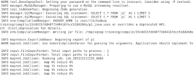
Sqoop is a handy tool to transfer bulk data between Hadoop and relational databases. It connects to MySQL via JDBC and automatically creates MapReduce functions with some simple commands. After MapReduce, the data from HDFS will be persistently and locally stored on MySQL.

# Use Sqoop to run MapReduce and export the tab delimited
# text file under specified directory to MySQL
sqoop export --username mysql-username --password mysql-pwd  \
    --export-dir myinput                    \
    --input-fields-terminated-by '\t'       \
    --input-lines-terminated-by '\n'        \
    --connect jdbc:mysql://localhost/test1  \
    --table purchases

On the client

Finally on the client installed with SAS, the PROC SQL’s pass-through mechanism will empower the user to explore or download the data stored in MySQL at the node, which will be free of any of the Hadoop’s constraints.

proc sql;    
   connect to mysql (user=mysql-username password=mysql-pwd server=mysqlserv database=test1 port=11021);
   select * from connection to mysql
       (select * from purchases limit 10000);
    disconnect from mysql;
quit;

PROC PLS and multicollinearity

Multicollinearity and its consequences

Multicollinearity usually brings significant challenges to a regression model by using either normal equation or gradient descent.

1. Invertible SSCP for normal equation

According to normal equation, the coefficients could be obtained by . If the SSCP turns to be singular and non-invertible due to multicollinearity, then the coefficients are theoretically not solvable.

2. Unstable solution for gradient descent

The gradient descent algorithm seeks to use iterative methods to minimize residual sum of squares (RSS). For example, as the plot above shows, if there is strong relationship between two regressors in a regression, many possible combinations of  and  lie along a narrow valley, which all corresponds to the minimal RSS. Thus  can be negative, positive or even zero, which becomes a confounding effect with respect to a stable model.

Partial Least Squares v.s. Principle Components Regression

The most direct way to deal with multicollinearity is to break down the regressors and construct new orthogonal variables. PLS and PCR are both dimension reduction methods that eliminate multicollinearity. The difference is that PLS also implements the response variable to select the new components. PLS is particularly useful in answering questions with multiple response variables. The PLS procedure in SAS is a powerful and flexible tool applying either PLS or PCR. One book, An Introduction to StatisticalLearning, suggests PCR over PLS.

While the supervised dimension reduction of PLS can reduce bias, it also has the potential to increase variance, so that the overall benefit of PLS relative to PCR is a wash.

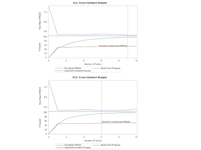
In the example using the baseball data set below, with 10-fold cross-validation, PLS chooses 9 components, while PCR picks out 5.

filename myfile url 'https://svn.r-project.org/ESS/trunk/fontlock-test/baseball.sas';
%include myfile;
proc contents data=baseball   position;
   ods output position = pos;
run;

proc sql;   
   select variable into: regressors separated by ' '
   from pos
   where num between 5 and 20;
quit;
%put ®ressors;

data baseball_t;
   set baseball;
      logsalary = log10(salary);
run;

proc pls data=baseball_t censcale nfac=10 cv=split(10);
   title 'partial least squares';
   model logsalary=®ressors;
run;

proc pls data=baseball_t censcale method = pcr nfac=10 cv=split(10);
   title 'princinple components regression';
   model logsalary=®ressors;
run;

Use R in Hadoop by streaming

It seems that the combination of R and Hadoop is a must-have toolkit for people working with both statistics and large data set.

An aggregation example

The Hadoop version used here is Cloudera’s CDH4, and the underlying Linux OS is CentOS 6. The data used is a simulated sales data set form a training course by Udacity. Format of each line of the data set is: date, time, store name, item description, cost and method of payment. The six fields are separated by tab. Only two fields, store and cost, are used to aggregate the cost by each store.

A typical MapReduce job contains two R scripts: Mapper.R and reducer.R.

Mapper.R

# Use batch mode under R (don't use the path like /usr/bin/R)  
#! /usr/bin/env Rscript  

options(warn=-1)  

# We need to input tab-separated file and output tab-separated file   

input = file("stdin", "r")  
while(length(currentLine = readLines(input, n=1, warn=FALSE)) > 0) {  
   fields = unlist(strsplit(currentLine, "\t"))  
   # Make sure the line has six fields  
   if (length(fields)==6) {  
       cat(fields[3], fields[5], "\n", sep="\t")  
   }  
}  
close(input)

Reducer.R

#! /usr/bin/env Rscript  

options(warn=-1)  
salesTotal = 0  
oldKey = ""  

# Loop around the data by the formats such as key-val pair  
input = file("stdin", "r")  
while(length(currentLine = readLines(input, n=1, warn=FALSE)) > 0) {  
  data_mapped = unlist(strsplit(currentLine, "\t"))  
  if (length(data_mapped) != 2) {  
    # Something has gone wrong. However, we can do nothing.  
    continue  
  }   

  thisKey = data_mapped[1]  
  thisSale = as.double(data_mapped[2])  

  if (!identical(oldKey, "") && !identical(oldKey, thisKey)) {  
    cat(oldKey, salesTotal, "\n", sep="\t")  
    oldKey = thisKey  
    salesTotal = 0  
  }  

  oldKey = thisKey  
  salesTotal = salesTotal + thisSale  
}  

if (!identical(oldKey, "")) {  
  cat(oldKey, salesTotal, "\n", sep="\t")  
}  

close(input)

Testing

Before running MapReduce, it is better to test the codes by some linux commands.

# Make R scripts executable   
chmod w+x mapper.R  
chmod w+x reducer.R  
ls -l  

# Strip out a small file to test   
head -500 purchases.txt > test1.txt  
cat test1.txt | ./mapper.R | sort | ./reducer.R

Execution

One way is to specify all the paths and therefore start the expected MapReduce job.

hadoop jar /usr/lib/hadoop-0.20-mapreduce/contrib/streaming/hadoop-streaming-2.0.0-mr1-cdh4.1.1.jar   
-mapper mapper.R –reducer reducer.R   
–file mapper.R –file reducer.R   
-input myinput  
-output joboutput

Or we can use the alias under CDH4, which saves a lot of typing.

hs mapper.R reducer.R myinput joboutput

Overall, the MapReduce job driven by R is performed smoothly. The Hadoop JobTracker can be used to monitor or diagnose the overall process.

Rhadoop or streaming?

RHadoop is a package developed under Revolution Alytics, which allows the users to apply MapReduce job directly in R and is surely a much more popular way to integrate R and Hadoop. However, this package currently undergoes fast evolution and requires complicated dependency. As an alternative, the functionality of streaming is embedded with Hadoop, and supports all programming languages including R. If the proper installation of RHadoop poses a challenge, then streaming is a good starting point.