The KFC toy problem: perspectives from four job roles

There is an interesting question —

There are 5 different types of toys at a KFC restaurant. If you go there, you will get one toy randomly. How many times do you need to go to KFC in order to get all 5 toys?

The question is about probabilistic analysis. Different professionals, such as a business analyst, a statistical programmer, a mathematician and a software developer, will have different thinking pathway to solve this problem. Let's see what they would think.

1. Business Analyst

A business analyst will tend to do scenario analysis at the first step.

Best-case scenario:

Assume I am so lucky that each time I visit KFC and get a different toy, then I only need 5 times to have all the five toys. The minimum number is 5.

Worst-case scenario:

To get a different toy I need to go to KFC five times. If there is not the toy I want, I will come back with empty hand. Thus, I will have to go to KFC 5*5 = 25 times. Of course, this scenario never happens.

OK. Then the mean times I need to go to KFC seems to be in a range [5, 25). Let's give the simplest try — use the (5+25)/2 to get 15 times. The number is not accurate but at least we have an estimate.

2. Statistical Programmer

As a brute-force tool, simulation is the instant thought for a statistical programmer. Let the computer randomly create 10,000 trials — say a person plays the game 10,000 times. After averaging the results, the computer eventually tells the expected times to get the 5 toys.

I modified the SAS code from a post by Rick Wicklin, and set the maximum number of visits to KFC as 32. After 10,000 runs, the mean is 11.37. The hunch tells that this number should be quite close.

************(1)Simulate 10000 trials**************************;
proc iml;
   K = 5; /* number of toys */
   L = 32; /* max visits per trial */
   /* generate NSim trials of L visits */
   NSim = 10000;
    x = j(Nsim, L);
   call randseed(12345);
   call randgen(x, "Uniform");
   x = ceil(K*x); /* integers in [1,K] */
   /* record the visit when 5 toys are taken */
   c = j(NSim,1,0); /** allocate */
    do i = 1 to NSim;
      do j = 5 to L;
         rowUnique = countunique(x[i, 1:j]);
         if rowUnique = 5 then do;
            c[i, 1] = j;
            goto skip;
         end;
      end;
      skip:
    end;
   /* output the result */
   create _1 from c;
      append from c;
   close _1;
;quit;

data _2;
   set _1;
   /* remove the trials that didn't get 5 toys in 32 visits */
   where col1 >= 5;
 run;
************(2)Show the results*******************************;
proc sgplot;
   density col1;
   density col1 / type = kernel;
run;

proc means;
run;

3. Mathematician

Actually this question is a variant of Coupon collector's problem. The mean/expectation and standard deviation can be derived directly by the formulas. The final expectation should be 5*(1+1/2+1/3+1/4+1/5) = 11.41. This is the answer.

4. Software Developer

A software developer considers time complexity and space complexity first. When N is approaching infinity, the question is similar to a merge sorting. Given a merge sort is O(nlog(n)), the expected times must be greater than 5*ln(5) = 8.05. At least this number will be a lower bound for this question.

Why sometimes use DATA Step instead of PROC SQL

A question

There is an interesting thread about the efficiency of PROC SQL on Mitbbs.com.

Both datasets have1 and have2 have few variables, but many observations. Very simple program, but without any result after running it for a whole afternoon.

proc sql;
    create table want as 
    select *
    from have1 as a left have2 as b
    on b.serie_beg <= a.serie <= b.serie_end;
quit;

If I replace left join with inner join, the result is the same. Why it takes so long?

Four types of joins in PROC SQL

To understand this question, we may have to go back into PROC SQL. A technical paper introduces that like other more generalized database systems, there are four kinds of joins to combine two data sets (tables) in the SQL procedure of SAS: Cartesian join, Hash join, Merge join and Indexed join. Using the command _method at the proc sql statement can let the log of SAS tell which join the current join is based on. For example, sqxjsl stands for Cartesian join; sqxjhsh is for Hash join; sqxjm is for Merge join; sqxjndx is for Indexed join.

• Cartesian join

Cartesian join uses two nested loops to join two tables. In other SQL systems, Cartesian join is often referred as Nested loop join. Suppose one table has N elements and the other has M elements, the complexity of this algorithm is , and is a bilateral merge that costs more resources. It can be shown in an example below.

************(0)Separate as 2 datasets***************;
data male female;
    set sashelp.class;
    if sex = 'F' then output female;
    else output male;
run;

************(1) Cartesian join ***************;
proc sql _method;
    create table friends1 as
    select a.name as name1, b.name as name2, a.age as age1, b.age as age2
    from male as a left join female as b on a.age > b.age
;quit;

The _method option outlines the execution plan of the join. Here this Cartesian join can't be replaced by more advanced join, and SAS honestly indicates that it is the only approach available.

NOTE: The execution of this query involves performing one or more Cartesian product joins that can not be optimized.

NOTE: SQL execution methods chosen are:

      sqxcrta
          sqxjsl
              sqxsrc( WORK.FEMALE(alias = B) )
              sqxsrc( WORK.MALE(alias = A) )

• Merge join

Merge join implements a sorting for each of the tables and merges them afterward. The time spent is the summation between the sorting and the scanning, and therefor the complexity is .

************(2) Merge join ***************;
proc sql _method;
    create table friends2 as
    select a.name as name1, b.name as name2, a.age as age1, b.age as age2
    from male as a left join female as b on a.age = b.age
;quit;

Clearly this join contains two sqxsort steps before the following sqxjm step. The logic here is quite similar to the traditional DATA Step's sort-sort-merge.

NOTE: SQL execution methods chosen are:

      sqxcrta
          sqxjm
              sqxsort
                  sqxsrc( WORK.FEMALE(alias = B) )
              sqxsort
                  sqxsrc( WORK.MALE(alias = A) )

• Hash join

Hash join loads the tables (if they are small enough to fit memory) into memory as hashs table and then do the scanning. The in-memory process is fast and the big O is .

************(3) Hash join ***************;
proc sql _method;
    create table friends3 as
    select a.name as name1, b.name as name2, a.age as age1, b.age as age2
    from male as a inner join female as b on a.age = b.age
;quit;

Usually such an inner join initiates the Hash join.

NOTE: SQL execution methods chosen are:

      sqxcrta
          sqxjhsh
              sqxsrc( WORK.MALE(alias = A) )
              sqxsrc( WORK.FEMALE(alias = B) )

• Indexed join

For relative large data sets that are frequently read, building an index is a good idea. An index is a basically a B-tree structure that translates to . If we have indexes for both lookup table and base table, the complexity will be like . In the demo below, I create two indexes for a lookup table and a simulated data set.

************(4) Indexed join ***************;
data simu;    
    do number = 1 to 1e6;
        output;
    end;
run;

proc sql _method;
    create index number on simu(number)
    ;
    create index age on male(age)
    ;
    create table friends4 as
    select a.name as name1, a.age as age1, b.number
    from male as a inner join simu as b on a.age = b.number
;quit;

Hereby the Indexed join has been automatically activated.

NOTE: SQL execution methods chosen are:

      sqxcrta
          sqxjndx
              sqxsrc( WORK.MALE(alias = A) )
              sqxsrc( WORK.SIMU(alias = B) )

Alternative solutions to the question

The good thing for PROC SQL is that the execution plan manager always chooses the optimized join plan. The bad thing is that the user is not allowed to specify any particular join. As for the question at the beginning, the Cartesian joins are obviously chosen to realize the left joins. If the data sets are quite large, the waiting seems to be painful. However, I can imagine some other ways in SAS to apply faster algorithms and avoid the Cartesian joins if not necessary.

• DATA Step Merge

The sort-sort-merge forces a merge join, which decreases the complexity from to .

• PROC FORMAT

If the lookup table is not very large, a user defined format with PROC FORMATis a unique way in SAS to construct the hash table in memory to perform lookup or scanning, which further decreases the complexity from to .

10 toughest interview questions for R developers (1)

I recently discovered 10 questions most daunting in R development, and I am trying to find the answers below.

1. Data structure -- How many data structures R has? How do you build a binary search tree in R?
2. Sorting -- How many sorting algorithms are available? Show me an example in R.
3. Low level -- How do you build a R function powered by C?
4. String -- How do you implement string operation in R?
5. Vectorization -- If you want to do Monte Carlo simulation by R, how do you improve the efficiency?
6. Function -- How do you take function as argument of another function? What is the apply() function family?
7. Threading -- How do you do multi-threading in R?
8. Memory limit and database -- What is the memory limit of R? How do you avoid it? How do you use SQL in R?
9. Testing -- How do you do testing and debugging in R?
10. Software development -- How do you develop a package? How do you do version control?

Q1. Data structure -- How many data structures R has? How do you build a binary search tree in R?
My answer: R mainly has 5 data structures.
Homogeneous(contain the same type of objects): vector --> matrix --> array
Heterogeneous(allow different type of objects): list --> data frame

A binary search tree requires several actions: implement a tree, insert nodes and delete nodes. We should create individual routines in R.

In R, a matrix is the ideal data structure to contain the linked elements. Then a list should be used to wrap the matrix and pass the arguments.

For insert-node routine, there is the pseudocode for it. The key point here is to use recursion in R’s function. Norman Matloff gave a complete example at page 180 of his book. 

insert(X, node){
 if(node = NULL)
 node = new binaryNode(X,NULL,NULL)
 return
 }
 if(X = node:data)
 return
 else if(X < node:data)
 insert(X, node:leftChild)
 else // X > node:data
 insert(X, node:rightChild)
}

Q2. Sorting -- How many sorting algorithms are available? Show me an example in R.
My answer: there are mainly 5 kinds of sorting algorithms(with their complexity):
Bubble Sort - O(n^2);
Selection Sort - O(n^2)
Merge Sort - O(n log n)
Quick Sort - from O(n log n) to O(n^2)
Bucket Sort - O(n + m)

R has a native sort function sort(), which is written by C and uses Quick Sort.

There is an example of Quick Sort in R by recursion

qs <- function(x) {
 if (length(x) <= 1) return(x)
 seed <- x[1]
 rest <- x[-1]
 sv1 <- rest[rest < seed]
 sv2 <- rest[rest >= seed]
 sv1 <- qs(sv1)
 sv2 <- qs(sv2)
 return(c(sv1,seed,sv2))
}

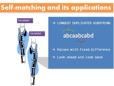
Self-matching and its applications

Programming is all about data structure and algorithm. For example, value comparison needs to find right data structure and iteration method. To fulfill this purpose, the first thing is to load the variable with a key-value like data structure, followed by key-driven iterations. In SAS, the typical key-value data types are array and hash table. Proc Format powered format can be another option. For data merging or equivalent values searching, those data types are pretty adequate. If exact numerical difference is desired, those SAS data structures may have some obstacles. First of all, array and hash table have to be created in a data step, which means they cannot be saved and reused, unless they are unidirectional translated to another data structure - dataset. Second, data loading is somewhat cumbersome: as for array, data has to be transposed to be assigned to an array; as for hash table, data step inherent iteration has to be carefully avoided and hash object still has limited methods.

Value comparison can utilize either data step's inherent iteration or SQL's Cartesian-product iteration. Explicit loops could be largely bypassed through these means. For instance, to remove unrelated adjacent numbers in a grouped data set, a strategy called ‘look-ahead and look-back’ is suggested by one blog post on SAS Community[1]. Several SAS-L users kindly provided answers for this specific question [2]. Within the four workable solutions, using data step, Arhur Tabachneck and BBSER2009 implemented the lagged or temporary variables derived from the same variable to compare values; Joe Matise and Bolotin Yevgeniy realized the same goal by Proc SQL (Example 1).

The strategy can be further extended to the cases requiring more iterations. In one real-world sample, to search values with fixed difference in a variable, a conditional self-matching SQL command can achieve n-choosing-2 comparisons simply and quickly(Example 2). Finding longest repeated substring is a famous algorithm question in computer science. And the common answer is to construct Suffix tree and look for the deepest node. In another example below, self-matching by Proc SQL can be a short-cut solution without considering many algorithm details (Example 3).

Self-matching is not the most efficient algorithm. Proc SQL is demanding on memory, while intensive data I/O can cause data step freezing. Arhur Tabachneck metioned that the application on large dataset may lead into SQL infinite loop [2], which I think as a stack overflow due to calling too much memory. However, in many scenarios of values comparison, using self-matching technique could dramatically decrease coding complexity and save time.

References: 1. 'Look-Ahead and Look-Back'. http://www.sascommunity.org/wiki/Look-Ahead_and_Look-Back.
2. 'Removing numbers'. http://www.listserv.uga.edu/cgi-bin/wa?A1=ind1101d&L=sas-l#44.

*********(1)EXAMPLE1 --  REMOVE UNRELATED NUMBERS WITHIN GROUPS*****;
******(1.0) INPUT OF THE RAW DATA******;
data one;
 input id:$1. var1 @@;
 cards;
a  4 b  2 b  3 b  4 b  8 b  9 b  10 b  11
b  13  b  15 b  16 c  1 c  2  c  5
;
run;

*******(1.1) ARTHUR TABACHNECK'S PLAN************;
data AT_RESULT (drop=prev_: next_:);
    set one;
    by id;
    set one ( firstobs = 2 keep = var1
            rename = (var1 = next_var1) )
    one ( obs = 1 drop = _all_ );
    prev_var1 = ifn( first.id, (.), lag(var1) );
    next_var1 = ifn(  last.id, (.), next_var1 );
    if abs(var1-prev_var1) eq 1 or
    abs(var1-next_var1) eq 1 then output;
run;

******(1.2) BBSER2009'S PLAN****;
data BBSER2009_RESULT(rename=(temp_id=id temp_var1=var1)) ;
      length pre_id $1;
      retain pre_id; retain pre_var1 .; retain pre_op 0;
      set one;
      if var1-pre_var1=1 then  do;
         if pre_op=0 then do;
    temp_id=pre_id;
    temp_var1=pre_var1;
    output;
    end;
        temp_id=id;
      temp_var1=var1;
    output;
        pre_op=1;
      end;
      else pre_op=0;
      pre_id=id; pre_var1=var1;
   keep temp_id temp_var1;
run;

********(1.3) JOE MATISE'S PLAN*************;
proc sql;
create table JM_RESULT  as
  select * from one h
  where exists (
      select 1 from one v
      where h.id=v.id
      and (h.var1 = v.var1-1
        or h.var1 = v.var1+1));
quit;

*******(1.4) BOLOTIN YEVGENIY'S PLAN*****;
proc sql;
  create table BY_RESULT as
       select distinct a.*
       from    one a
               inner join one b
       on a.id = b.id
       where abs(a.var1 - b.var1)=1;
quit;

*********END OF EXAMPLE (1)**********;

*******(2) EXAMPEL 2 -- FIND ANY VALUES WITH FIXED DIFFERENCES****** ;
*****(2.1) INPUT RAW DATA******;
data timeseries;
    input  date1 date9.  var1;
    cards;
    11jan2008  11
    12jan2008 10
    13jan2008 21
    14jan2008 20
    15jan2008 30
    16jan2008 30
;
run;

*****(2.2) FIND ALL DATES WITH UNTI DIFFERENC EQUALS 10****;
proc sql;
    create table timeseries1 as
    select a.date1 as date1 format=date9., a.var1 as unit1, b.date1 as date2 format=date9., b.var1 as unit2
    from timeseries as a, timeseries as b
    where a.var1-b.var1=10
;quit;

****END OF EXAMPLE (2)**********;

****(3) EXAMPLE3 --  FIND LONGEST DUPLICATED SUBSTRING SEARCH****;
***(3.0) INPUTRAW DATA***;
data test(where=(missing(char)=0));
   input char $1.@@;
    id=_n_;
   cards;
abcaabcabd
;
run;

***(3.1) SINGLE CHARACTER MATCHING****;
proc sql;
    create table test1 as
    select  a.id as id1, b.id as id2, a.char as char1, b.char as char2, 
            abs(id1-id2) as pos
    from test as a, test as b
    where a.char=b.char and id1 lt id2
    order by pos, id1
;quit;

****(3.2) REMOVE ONE-CHARACTER DUPLICATES****;
data test2;
  set test1;
  by pos;
  dif = dif(id1);
  if first.pos then dif=1;
  if dif eq 1;
  if first.pos and last.pos then delete;
run;

****(3.3) CONCATENATING DUPLICATES****;
proc transpose data=test2 out=test3;
    by pos ; 
    var char1;
    run;
    
data test4;
    set test3;
    array allvar[*] col:;
    repeat = cats(of allvar[*]);
run;

****(3.4) SHOW THE LONGEST DUPLICATED SUBSTRING****;
proc sql;
    select max(repeat) 'The longest duplicated substring'
    from test4
;quit;

******END OF EXAMPLE(3)****************;

*****(4) EXAMPLE 4 -- FIND THE PRODUCT FROM ANY TWO NUMBERS IN AN ARRAY***

data have;    
    input var1;
    cards;
    1
    -3 
    3
    9
    12
    23
    34
    5
    8
    9
    -5
    ;
run;

data temp;
    set have;
    idx = _n_;
run;

proc sql;
    create table want as
    select a.var1 * b.var1 as product
    from temp as a, temp as b
    where a.idx ne b.idx
;quit;
**************END OF EXAMPLE 4**********;