SAS and Revolution R for GB size data

R surpassed Matlab and SAS on recent Tiobe Programming index for popularity. I agree with this ranking[1], since R could largely replace Matlab and SAS for MB size data, and it is getting hot. The fast growing sectors, quantitative finance, bioinformatics and web analytics, are all embracing R. In those competitive fields, survival demands the skills of a developer instead of a programmer, which suggests something brings more power or higher AUC. The cross-platform, open-sourced, C-based, function-friendly R is right on top of the tide. SAS programmers have to wait SAS Institute to build tools for them, while an R developer could invent his own gloves and axes. SAS’s licensing policy is also problematic: SAS is divided into modules, such as BASE, STAT, IML, GRAPH, ETS, etc; if you want to use just one procedure in a module, you should buy the whole module and renew the license each year. Norman Nie[2] said that 15 core statistical procedures, such as cluster analysis, factor analysis, PCA and Cox regression, would satisfy 85% of the needs. Thus SAS programmers may have to pay the cost of hundreds of procedures to use the 15 procedures. On the contrary, you can specify and download any package for R. Or you construct brand-new functions or packages.

However, with larger data, R or Matlab users have to painfully jump to low-level languages. For convenience of matrix computation, R or Matlab routinely keeps copies of data in memory and does not let garbage collector frenetically dump them. With GB size data, people would soon hear the outcry of memory shortage in their workstation, and ponder to resort to C or C++. That is possibly why Matlab or R talents are so popular in academia but never welcome in job market. Amazingly, SAS is pretty robust to deal with this scale of data. SAS rarely failed me even though I sometimes complain about the speed. Of course, if memory is not a hurdle, R is another good option. Inspired by this idea, Norman Nie‘s startup company Revolution Analytics reinvigorated the community R. They used an XDF data file on hard disk to contain data before into memory stack. Then their unique package RevoScaleR would perform data analysis inside of those files. This strategy is pretty similar to the In-Database technology by SAS’s high-end enterprise products. Besides, XDF would forcibly partition data to allow multiple-core processing. On a common PC with 3G memory, I compared Revolution R and SAS using a 1.1 GB flat file. SAS integrated it in 20 seconds, while Rev R did that in 5 minutes. Afterward SAS realized some data transformation steps and summarization procedures. Unfortunately in those occasions the R core of Rev R usually crashed with the Rev R’s IDE left as a zombie. Presumably the compatibility between the R core and the XDF file system is a concern. In addition, at this stage the RevoScaleR package in Rev R has limited functions or procedures, such as summary statistics, linear regression, logistic regression, cross-tab, which utilized the advantage of the XDF system. Another worry is that the R core contributors, led by Ross Ihaka and Robert Gentleman, may feel reluctant to further assist Norman Nie's effort to develop his profitable product.

For TB size data, R will roll back. Like the physical world with extraordinary speed or space that Newton's theories expire, the complex, high-volume, high-dimensional data would stun any extraction, transformation, loading and analysis operations base on the concept of RDBMS. MySQL, Oracle and SAS all fade away. Distributed system and function languages are the rescue. Open source software, like Python and R, rule in this domain. The data center would aggregate the total memory from thousands of servers. With gigantic memories all together, data analysis by R could be performed by scheduling a Map/Reduce task. However, those well-known IT giants owning those data centers are not likely to buy many licenses for a commercial package. The community R, not Revolution R, will enjoy a significant share from the rapid growth in this area.

Overall SAS is still much better than Revolution R in handling GB size data now. Revolution R may need more time to get matured for production purpose. Revolution R launched a SAS-to-R challenge and deliberately created a function to transform SAS datasets to its XDF format. I like to see newcomers in the arena, and SAS may benefit from this competition.

Reference: 1. 'TIOBE Programming Community Index for February 2011'. http://www.tiobe.com/index.php/content/paperinfo/tpci/index.html
2. 'Another Open Source Swipe at IBM and SAS'. http://blogs.forbes.com/quentinhardy/2011/02/01/another-open-source-swipe-at-ibm-and-sas/

************(1) DOWNLOAD AND UNZIP THE DATA ***********************;
ftp://ftp.cdc.gov/pub/Health_Statistics/NCHS/Datasets/DVS/mortality/mort2006us.zip

***********(2)SAS'S CODE TO INTEGRATE DATA*****************;
data mort06;
 infile 'C:\mort06.dat' 
    lrecl=150 missover ;
 input    @20 Resident_status     $1. 
    @83 Plac_of_death_decedent_status   $1.  
    @85 Day_of_week _of_death   $1. 
    @94 Date_receipt    $8.  
    @102 Data_Year     $4. 
    @65 Month_of_Death     $2.
    @60 Sex      $1.  
    @445 Race      $6.
    @70 Age      $13.  
    @84 Marital      $1.  
    @484 Hispanic_origin     $5.  
    @61 Education             $4.  
    @146 ICD10 $4.  
    @150 code358    $3.   
    @154 code113 $3.     
    @157 code130 $3.    
    @160 cause_recode   $2.   
    @145 Place_injury   $1.   
    @106 Injury_work     $1.  
    @108 Method_disposition    $1. 
    @109 Autopsy      $1. 
    @144 Activity    $1. 
;
run;

proc contents data=mort06;
run;

############(3) REV R 'S CODE TO INTEGRATE DATA#####################
colList <- list(  
    "Resident_status"        =list(type="factor",  start=20, width=1 ),
     "Plac_of_death_decedent_status"    =list(type="factor", start=83, width=1 ),
     "Day_of_week _of_death"      =list(type="factor", start=85, width=1 ),     
     "Date_receipt"         =list(type="factor", start=94, width=1 ),         
     "Data_Year"         =list(type="factor",  start=102, width=4  ),
     "Month_of_Death"        =list(type="factor", start=65, width=2  ),
     "Sex"           =list(type="factor", start=60, width=1  ),
     "Race"           =list(type="factor", start=445, width=6 ),
     "Age"           =list(type="factor", start=70, width=13  ),
     "Marital"          =list(type="factor", start=84, width=1 ),
     "Hispanic_origin"        =list(type="factor", start=484, width=5  ),
     "Education"         =list(type="factor", start=61, width=4 ),
     "ICD10"          =list(type="factor", start=146, width=4  ),     
     "code358"          =list(type="factor", start=150, width=3  ), 
     "code113"          =list(type="factor", start=154, width=3  ),
     "code130"          =list(type="factor", start=157, width=3  ),
     "cause_recode "        =list(type="factor", start=160, width=2  ),
     "Place_injury"         =list(type="factor", start=145, width=1  ),
     "Injury_work "         =list(type="factor", start=106, width=1  ),
     "Method_disposition"       =list(type="factor", start=108, width=1  ),
     "Autopsy"          =list(type="factor", start=109, width=1  ),
     "Activity"          =list(type="factor", start=144, width=1  )  
    )
mortFile <- file.path("C:", "MORT06.DAT")
sourceData <- RxTextData(mortFile, colInfo=colList )                 
outputData <- RxXdfData("MORT")
rxImportToXdf(sourceData, outputData,  overwrite = TRUE) 
rxGetInfoXdf("MORT.xdf", getVarInfo=TRUE) 

#################END OF CODING#######################################;  

Visualize decision tree by coding Proc Arboretum

Decision tree (tree-based partition or recursive partition) dominates the top positions of recent data mining competitions. It is easy to realize and explain like logistic regression, but usually brings more powers (AUC). Not like SVM, neural network or random forest, decision tree is quick and resource-efficient. It is really a blessing for big data. No wonder regression tree and classification tree are widely used in industry: thanks to Google’s application on its Gmail, I am seldomly harassed by spam.

The documents about Proc Arboretum are still scarce. From my experience, Proc Arboretum is pretty robust and powerful. It divides input variables as different categories: nominal/interval/interval. It allows users to trim the tree interactively. It also generates a number of statistics about portioning criterion. And it supports an integrated training-validation-scoring flow and even code output. Overall, it satisfies my wildest dream about decision tree. However, since it is one of the pillars of SAS Enterprise Miner, SAS Institute probably feels reluctant to disclose more detail of this procedure to those who have the license and are more willing to do hard coding themselves. SAS programmers can hardly build physical tree it if without Enterprise Miner. Some resort to R instead, because R’s package ‘rpart’ is now stable for production purpose and provides convenient functions to show the trees.

SAS’s plotting procedures could visualize the results by Proc Arboretum. In the example, I still used the example SASHELP.CARS to explore if the decision tee recognizes the origin of a car, such as Asia/Europe/US. With an ancient procedure Proc Netdraw, I built a not-good-looking tree. By other high-level plotting SG procedures, I displayed some deeper information according to the results by Proc Arboretum, such as the significance of variables or the predication accuracy.

Reference: The ARBORETUM Procedure. 'www.sasenterpriseminer.com/documents/proc_arbor.pdf'.

********(1) CONSTRUCT DECISION TREE AND OUTPUT DATASETS********;
filename outcode 'h:\outcode.txt';
proc arboretum data=sashelp.cars ;
    target origin / level=nominal;
    input MSRP Cylinders Length  Wheelbase MPG_City 
    MPG_Highway Invoice Weight Horsepower/ level=interval;
    input EngineSize/level=ordinal;
    input  DriveTrain Type /level=nominal;
    code file=outcode;
    save   IMPORTANCE=imp1 MODEL=model1  NODESTATS=nodstat1  
    RULES=rul1 SEQUENCE=seq1  STATSBYNODE= statb1 SUM=sum1;
run;
quit;
********END OF STEP(1)***********;

********(2) VISUALIZE DECISION TREE RESULTS************;
****(2.1) SIGNIFICANCE OF VARIABLES*****;
proc sgplot data=imp1;
    vbar name/response=importance;
run;

****(2.2) INTERACTION AMONG THE MOST THREE SIGNIFICANT VARIABLES****;
proc sgscatter data=sashelp.cars;
    plot  invoice*(wheelbase length)/group=origin;
run;

****(2.3) CONSTITUENTS OF EACH NODE****;
proc sgplot data=statb1;
    vbar node/response=STATVALUE group=CATEGORY;
run;

****(2.4) BUILD PHYSICAL TREE****;
proc sql;
    create table treedata as
    select a.parent as act1, a.node, b.NODETEXT, b.U_Origin
    from nodstat1 as a, nodstat1 as b
    where a.parent=b.node
    union
    select c.node as act1, . as node, c.nodetext, c.U_Origin
    from nodstat1 as c
;quit;

data treedata1;
    set treedata;
    if U_Origin='Asia' then _pattern=1;
    else if U_Origin='Europe' then _pattern=2;
    else  _pattern=3;
run;

pattern1  c=green; pattern2 v=s c=red;  pattern3 v=s c=blue; 
/*NOTE: USE PROC NETDRAW TO REALIZE PHYSICAL TREE*/
footnote   c=green   'Asia  '  c=red     'Europe '    c=blue    'USA'; 
proc netdraw data=treedata1 graphics; 
     actnet /activity=act1 successor=NODE  id=(NODETEXT) tree compress rotate     rotatetext font=simplex arrowhead=0 htext=6; 
run;
footnote ' ';

****(2.5) SHOW ALL PARTITION STATISTICS *****;
proc transpose data=seq1 out=seq1_t(rename=(col1=value));
    var _ASSESS_  _MISC_ _MAX_  _SSE_  _ASE_;
    by _NW_  notsorted;
run; 
      
proc sgpanel data=seq1_t;
    panelby _name_/UNISCALE=column COLUMNS=4 rows=2 SPACING=5 NOVARNAME;
        step x=_NW_  y=value;
    colaxis TYPE= DISCRETE grid;
run; 

****(2.6) SHOW FINAL PREDICATION ACCURACY****;  
proc sort data=sum1( drop=_total_) out=sum1_s;
    by _TARGET_;
    where _STAT_='N' AND _TARGET_ ^= 'TOTAL';
run;

proc transpose data=sum1_s out=sum1_t(rename=(col1=Number));
    var _numeric_;
    by _TARGET_;
run;

proc sgplot data=sum1_t;
    vbar _LABEL_/response=Number group=_TARGET_;
run;
********END OF STEP(2)*********;

*********END OF ALL CODING*****TESTED ON PC SAS 9.2 ***********;

Use Python to normalize database

Many occasions, data needs to be normalized to speed up query operations before entering a database. Large text files have to depend on Python, given its’ excellent row-wise data manipulation ability.

First thought is to use a nested list to fill in all the data, such as the codes below.

import csv, sqlite3

infile = open('mtcars.csv', 'r')
f = csv.reader(infile)
header = f.next()
header.pop(0)

data = [] 
for r in f:
    name = r.pop(0)
    for i in range(0, len(r)):
        data.append([name, header[i], r[i]])

However, a dictionary will be much more convenient given its built-in iteration tools.

import csv, sqlite3

infile = open('mtcars.csv', 'r')
f = csv.DictReader(infile)

data = [] 
for r in f:
    a = r.popitem()[1]
    for key, value in r.iteritems():
        data.append([a, key, float(value)])

infile.close()

# Create an empty table for the codes below
db = sqlite3.connect('mtcars.db')
c = db.cursor()
c.execute('create table if not exists display(name text, varname text, varvalue real) ')
db.commit()

# Insert the normalized data into SQLite database 
c.executemany('insert into display values (?, ?, ?)', data)
db.commit()

# Show the result
for row in c.execute('select * from display'):
    print row

Proc Fcmp(4): Binomial tree vs. Black-Scholes model

  
The very truth is that SAS has limited financial functions. Thanks to SAS Institute, they finally added some option pricing functions in the base module of SAS 9.2, such as Black-Scholes put/call functions, Garman-Kohlhagen put/call functions, etc. Thus, the number of financial functions in the SAS toolbox adds up to more than 20 now.

Functions made easy by Proc Fcmp. In the finance’s brave new world of functions, financial function is ammo in a war. A unique and resourceful stockpile of functions is desired. Previously, in SAS, macro may seem like a reasonable substitute. However, when we deal with situations like evaluating y=h(x1)*f(x2), macro is feeble. The new procedure debuted in SAS 9.2, Proc Fcmp, provides us an easy way to create and accumulate functions, which will benefit people who are struggling to use SAS to solve finance problems in Data Step.

Proc Fcmp is used for a Binomial tree function of European call option pricing in this example. Once set up, it is very handy to use a function in the common Data Step: the function just acts like an inherent one. In the example, the exercise price ‘E’ is 50, the time to maturation 't' is 5 months, the share price ‘S’ is 50 again, the risk-free interest rate ‘r’ during t is 0.05, and the volatility ‘sigma’ is 0.3. Then the SAS native Black-Scholes option call function ‘blkshclprc’ and the newly ‘manufactured’ Binomial tree function ‘Eurocall’ powered by Proc Fcmp are compared. With the increasing of the layers ‘n’ of the Binomial tree model or the expanding of the tree branches, the option price fluctuates and gets closer to the price by Black-Scholes model. Finally it may converge to the ‘correct’ price. The results show that more steps may provide more accurate result for a Binomial tree model.

Everything in Proc Fcmp is encapsulated. Typically in designing a macro, we concern about the local or global variables. While dealing with a function by Proc Fcmp, it is argument in and argument out: no variable in a function would leak. All arrays in Proc Fcmp are also temporary unless they are indicated as output. Those features are friendly in making a workable function rapidly.

Reference: 1. Paolo Brandimarte. Numerical Methods in Finance and Economics: A MATLAB-Based Introduction. Wiley-Interscience, 2006.
2. SAS 9.2 Language Reference: Dictionary, Third Edition. SAS Publishing. 2009.

proc fcmp outlib = myfunc.finance.price;
    function Eurocall(E, t, F, r, sigma, N);
        deltaT=T/N;
        u=exp(sigma*sqrt(deltaT));
        d=1/u;
        p=(exp(r*deltaT)-d)/(u-d);
        array tree[1]/ nosymbols;
        call dynamic_array(tree, n+1, n+1);
        call zeromatrix(tree);
        
        do i=0 to N;
            tree[i+1,N+1]=max(0 , E*(u**i)*(d**(N-i)) - F);
        end;
        do j=(N-1) to 0 by -1;
            do  i=0 to j by 1;
                tree[i+1,j+1] = exp(-r*deltaT)* 
                        (p * tree[i+2,j+2] + (1-p) * tree[i+1,j+2]);
            end;  
        end;
        price = tree[1,1];
        return(price);
    endsub;
run;


*****(2)Use Binomial tree model and Black-Scholes model functions *****;
options cmplib = (myfunc.finance);
data test;
    BSprice=blkshclprc(50, 5/12, 50, 0.05, 0.3);
    do n=1 to 100;
        Treeprice=eurocall(50, 5/12, 50, 0.05, 0.3, n);
        output;
    end;
run;

***********(3)Display the comparision between the two functions***************;
proc sgplot data=test;
    title 'The comparison between Black-Sholes model and Binomial tree model';
    needle x=n y=Treeprice/baseline=4;
    series x=n y=BSprice/ lineattrs=(color=red);
    yaxis label='Option price';
run;
***************END***************TEST PASSED 12DEC2010**************;

Macro embedded function finds AUC

As a routine practice to reuse codes, SAS programmers tend to contain procedures in a SAS macro and pass arguments to them as macro variables. The result could be anything by data set and SAS procedure: figure, dataset, SAS list, etc. Thus, macro in SAS is like module or class in other languages. However, if repeated calling of a macro is about to accumulate some key values based on different input variables, the design of such a macro could be tricky. My first thought is to use a nested macro (child macro within parent macro) to capture the invisible macro variables floating everywhere in the environment. The idea is pretty daunting, since I have to consider the scopes of macro variables from different macro layers and naming of temporary datasets.

Now with Proc Fcmp, macro embedded function allows the utilization of SAS’s procedure within Data Step. One of the unique features inProc Fcmp is that it could encapsulate macros by its RUN_MACRO function and RC handle. Implementation of macro embedded function has some advantages. First, since a self-defined function is called in a data step, all values would be automatically saved in the dataset of this data step. Second, we can just keep the exactly return values we want. The ODS statement first specifies the output dataset to be temporally saved. Then the exact value as a macro variable will be transported to function as return argument. Third, Proc Fcmp would provide an exception-handling mechanism, depending on the macro’s output. In this post, I showed one example with a SAS help file ‘SASHELP.CARS’ (code below). This dataset has the information of some car models. I would like to see which variables, such as car’s length, weight, price, etc, could predict whether this car is made by US or NON-US countries. Values of AUC (area under ROC curve) from logistic regression were obtained and compared by this strategy.

The user-defined function library is accessible and reusable. SAS provides a four-level directory to save user-defined functions (library-1st level directory- 2nd level directory –function’s name), and also a two-level directory for a complied macro (library-macro’s name). As for a macro embedded function, the complied macros and functions should be stored together at the same place. Then next time, by specifying the path in SAS option statement, those functions can be instantly invoked.

Reference: Stacey and Jacques. Adding Statistical Functionality to the DATA Step with PROC FCMP. SAS Global 2010.

******(1) CREATE COMPLIED MACRO AND FUNCTION******;
****(1.0) SET A PATH TO STORE MACRO AND FUNCTION***;
libname myfunc 'h:\myfun';
option  mstored sasmstore=myfunc;

****(1.1) CREATE THE EMBEDDED MACRO*****;
%macro auc_logis_macro() /store source des='auc_logis_macro';
    /* NOTE: DEQUOTE THE INPUT STRINGS */
 %let ds_in = %sysfunc(dequote(&ds_in));
 %let target = %sysfunc(dequote(&target));
 %let input = %sysfunc(dequote(&input));
 /* NOTE: USE PROC LOGISTIC TO GENERATE AUC */
 ods graphics;
 ods output Association= temp;
 ods select association roccurve;
 proc logistic data=&ds_in descending plots(only)=roc ;
  model &target = &input  ; 
 run;
    ods graphics off;
 /*NOTE: ONLY CHOOSE AUC TO OUTPUT  */
 proc sql noprint;
  select nValue2 into: auc_value
  from temp
  where Label2 = 'c'
 ;quit;
 /*NOTE: KILL THE INTERIM DATASET  */
 proc datasets; delete temp;run;
%mend auc_logis_macro;

****(1.2) INCORPORATE MACRO INTO FUNCTION ****;
proc fcmp outlib = myfunc.macro.functions;
   function auc_logis(ds_in $, target $ , input $);
      rc = run_macro('auc_logis_macro', ds_in, target, input, auc_value);
      if rc eq 0 then return(auc_value);
      else return(.);
   endsub;
run;
*******END OF STEP (1)***********;


*****(2) USE THE MACRO EMBEDDED FUNCTION*******;
****(2.0) FIND PATH FOR STORED FUNCTION AND MACRO****;
libname myfunc 'h:\myfun';
option cmplib = (myfunc.macro) mstored sasmstore=myfunc mprint symbolgen;

****(2.1) CREATE A BINARY TARGET VAR FROM A SAS HELP DATASET****;
data test;
 set sashelp.cars;
 length country  $6;
 if origin = 'USA' then country = 'US';
 else country = 'NON-US';
run;

****(2.2) INVOKE THE FUNCTION TO EVALUATE MULTIPLE VARS OR VARS' COMBINATION****;
data auc_ds;
  ds_in='test';
  target = 'country';
  length input $70;
 do input = ' Weight' , ' Length', 'Horsepower', 'EngineSize',  'MPG_City', 
'Wheelbase', 'Weight Length', ' EngineSize Weight Length MPG_City Wheelbase Horsepower MPG_Highway';
  auc=auc_logis(ds_in ,target,  input); OUTPUT;
 end;
run;

****(2.3) COMPARE ALL AUC VALUES****;
data auc_ds1;
 set auc_ds;
 label auc ='AUC';
 if _n_=8 then input ='All numeric variables';
run;
proc sgplot data=auc_ds1;
 vbar input/response=auc;
 yaxis grid;
 refline 0.5;
run;

****END OF STEP (2)****;
*****************END OF THE PROGRAM************;
 

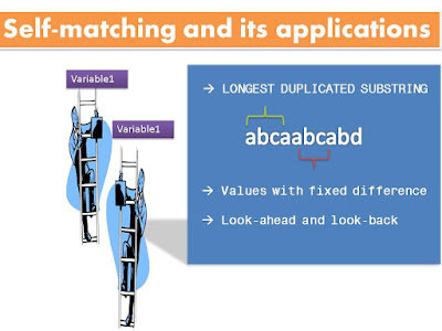
Self-matching and its applications

Programming is all about data structure and algorithm. For example, value comparison needs to find right data structure and iteration method. To fulfill this purpose, the first thing is to load the variable with a key-value like data structure, followed by key-driven iterations. In SAS, the typical key-value data types are array and hash table. Proc Format powered format can be another option. For data merging or equivalent values searching, those data types are pretty adequate. If exact numerical difference is desired, those SAS data structures may have some obstacles. First of all, array and hash table have to be created in a data step, which means they cannot be saved and reused, unless they are unidirectional translated to another data structure - dataset. Second, data loading is somewhat cumbersome: as for array, data has to be transposed to be assigned to an array; as for hash table, data step inherent iteration has to be carefully avoided and hash object still has limited methods.

Value comparison can utilize either data step's inherent iteration or SQL's Cartesian-product iteration. Explicit loops could be largely bypassed through these means. For instance, to remove unrelated adjacent numbers in a grouped data set, a strategy called ‘look-ahead and look-back’ is suggested by one blog post on SAS Community[1]. Several SAS-L users kindly provided answers for this specific question [2]. Within the four workable solutions, using data step, Arhur Tabachneck and BBSER2009 implemented the lagged or temporary variables derived from the same variable to compare values; Joe Matise and Bolotin Yevgeniy realized the same goal by Proc SQL (Example 1).

The strategy can be further extended to the cases requiring more iterations. In one real-world sample, to search values with fixed difference in a variable, a conditional self-matching SQL command can achieve n-choosing-2 comparisons simply and quickly(Example 2). Finding longest repeated substring is a famous algorithm question in computer science. And the common answer is to construct Suffix tree and look for the deepest node. In another example below, self-matching by Proc SQL can be a short-cut solution without considering many algorithm details (Example 3).

Self-matching is not the most efficient algorithm. Proc SQL is demanding on memory, while intensive data I/O can cause data step freezing. Arhur Tabachneck metioned that the application on large dataset may lead into SQL infinite loop [2], which I think as a stack overflow due to calling too much memory. However, in many scenarios of values comparison, using self-matching technique could dramatically decrease coding complexity and save time.

References: 1. 'Look-Ahead and Look-Back'. http://www.sascommunity.org/wiki/Look-Ahead_and_Look-Back.
2. 'Removing numbers'. http://www.listserv.uga.edu/cgi-bin/wa?A1=ind1101d&L=sas-l#44.

*********(1)EXAMPLE1 --  REMOVE UNRELATED NUMBERS WITHIN GROUPS*****;
******(1.0) INPUT OF THE RAW DATA******;
data one;
 input id:$1. var1 @@;
 cards;
a  4 b  2 b  3 b  4 b  8 b  9 b  10 b  11
b  13  b  15 b  16 c  1 c  2  c  5
;
run;

*******(1.1) ARTHUR TABACHNECK'S PLAN************;
data AT_RESULT (drop=prev_: next_:);
    set one;
    by id;
    set one ( firstobs = 2 keep = var1
            rename = (var1 = next_var1) )
    one ( obs = 1 drop = _all_ );
    prev_var1 = ifn( first.id, (.), lag(var1) );
    next_var1 = ifn(  last.id, (.), next_var1 );
    if abs(var1-prev_var1) eq 1 or
    abs(var1-next_var1) eq 1 then output;
run;

******(1.2) BBSER2009'S PLAN****;
data BBSER2009_RESULT(rename=(temp_id=id temp_var1=var1)) ;
      length pre_id $1;
      retain pre_id; retain pre_var1 .; retain pre_op 0;
      set one;
      if var1-pre_var1=1 then  do;
         if pre_op=0 then do;
    temp_id=pre_id;
    temp_var1=pre_var1;
    output;
    end;
        temp_id=id;
      temp_var1=var1;
    output;
        pre_op=1;
      end;
      else pre_op=0;
      pre_id=id; pre_var1=var1;
   keep temp_id temp_var1;
run;

********(1.3) JOE MATISE'S PLAN*************;
proc sql;
create table JM_RESULT  as
  select * from one h
  where exists (
      select 1 from one v
      where h.id=v.id
      and (h.var1 = v.var1-1
        or h.var1 = v.var1+1));
quit;

*******(1.4) BOLOTIN YEVGENIY'S PLAN*****;
proc sql;
  create table BY_RESULT as
       select distinct a.*
       from    one a
               inner join one b
       on a.id = b.id
       where abs(a.var1 - b.var1)=1;
quit;

*********END OF EXAMPLE (1)**********;

*******(2) EXAMPEL 2 -- FIND ANY VALUES WITH FIXED DIFFERENCES****** ;
*****(2.1) INPUT RAW DATA******;
data timeseries;
    input  date1 date9.  var1;
    cards;
    11jan2008  11
    12jan2008 10
    13jan2008 21
    14jan2008 20
    15jan2008 30
    16jan2008 30
;
run;

*****(2.2) FIND ALL DATES WITH UNTI DIFFERENC EQUALS 10****;
proc sql;
    create table timeseries1 as
    select a.date1 as date1 format=date9., a.var1 as unit1, b.date1 as date2 format=date9., b.var1 as unit2
    from timeseries as a, timeseries as b
    where a.var1-b.var1=10
;quit;

****END OF EXAMPLE (2)**********;

****(3) EXAMPLE3 --  FIND LONGEST DUPLICATED SUBSTRING SEARCH****;
***(3.0) INPUTRAW DATA***;
data test(where=(missing(char)=0));
   input char $1.@@;
    id=_n_;
   cards;
abcaabcabd
;
run;

***(3.1) SINGLE CHARACTER MATCHING****;
proc sql;
    create table test1 as
    select  a.id as id1, b.id as id2, a.char as char1, b.char as char2, 
            abs(id1-id2) as pos
    from test as a, test as b
    where a.char=b.char and id1 lt id2
    order by pos, id1
;quit;

****(3.2) REMOVE ONE-CHARACTER DUPLICATES****;
data test2;
  set test1;
  by pos;
  dif = dif(id1);
  if first.pos then dif=1;
  if dif eq 1;
  if first.pos and last.pos then delete;
run;

****(3.3) CONCATENATING DUPLICATES****;
proc transpose data=test2 out=test3;
    by pos ; 
    var char1;
    run;
    
data test4;
    set test3;
    array allvar[*] col:;
    repeat = cats(of allvar[*]);
run;

****(3.4) SHOW THE LONGEST DUPLICATED SUBSTRING****;
proc sql;
    select max(repeat) 'The longest duplicated substring'
    from test4
;quit;

******END OF EXAMPLE(3)****************;

*****(4) EXAMPLE 4 -- FIND THE PRODUCT FROM ANY TWO NUMBERS IN AN ARRAY***

data have;    
    input var1;
    cards;
    1
    -3 
    3
    9
    12
    23
    34
    5
    8
    9
    -5
    ;
run;

data temp;
    set have;
    idx = _n_;
run;

proc sql;
    create table want as
    select a.var1 * b.var1 as product
    from temp as a, temp as b
    where a.idx ne b.idx
;quit;
**************END OF EXAMPLE 4**********;