An alternative way to use SAS and Hadoop together

The challenges for SAS in Hadoop

For analytics tasks on the data stored on Hadoop, Python or R are freewares and easily installed in each data node of a Hadoop cluster. Then some open source frameworks for Python and R, or the simple Hadoop streaming would utilize the full strength of them on Hadoop. On the contrary, SAS is a proprietary software. A company may be reluctant to buy many yearly-expired licenses for a Hadoop cluster that is built on cheap commodity hardwares, and a cluster administrator will feel technically difficult to implement SAS for hundreds of the nodes. Therefore, the traditional ETL pipeline to pull data (when the data is not really big) from server to client could be a better choice for SAS, which is most commonly seen on a platform such as Windows/Unix/Mainframe instead of Linux. The new PROC HADOOP and SAS/ACCESS interface seem to be based on this idea.

Pull data through MySQL and Sqoop

Since SAS 9.3M2, PROC HADOOP can bring data from the cluster to the client by its HDFS statment. However, there are two concerns: first the data by PROC HADOOP will be unstructured out of Hadoop; second it is sometimes not necessary to load several GB size data into SAS at the beginning. Since Hadoop and SAS both have good connectivity with MySQL, MySQL can be used as an middleware o communicate them, which may ease the concerns above.

On the Cluster

The Hadoop edition used for this experiment is Cloudera’s CDH4. The data set, purchases.txt is a tab delimited text file by a training course at Udacity. At any data node of a Hadoop cluster, the data transferring work should be carried out.

MySQL

First the schema of the target table has to be set up before Sqoop enforces the insert operations.

# Check the head of the text file that is imported on Hadoop
hadoop fs -cat myinput\purchases.txt | head -5

# Set up the database and table 
mysql --username mysql-username --password mysql-pwd
create database test1;
create table purchases (date varchar(10), time varchar(10), store varchar(20), item varchar(20), price decimal(7,2), method varchar(20));

Sqoop

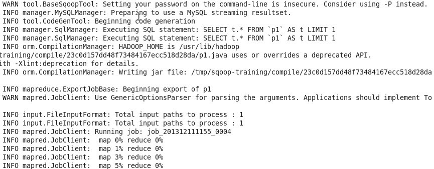
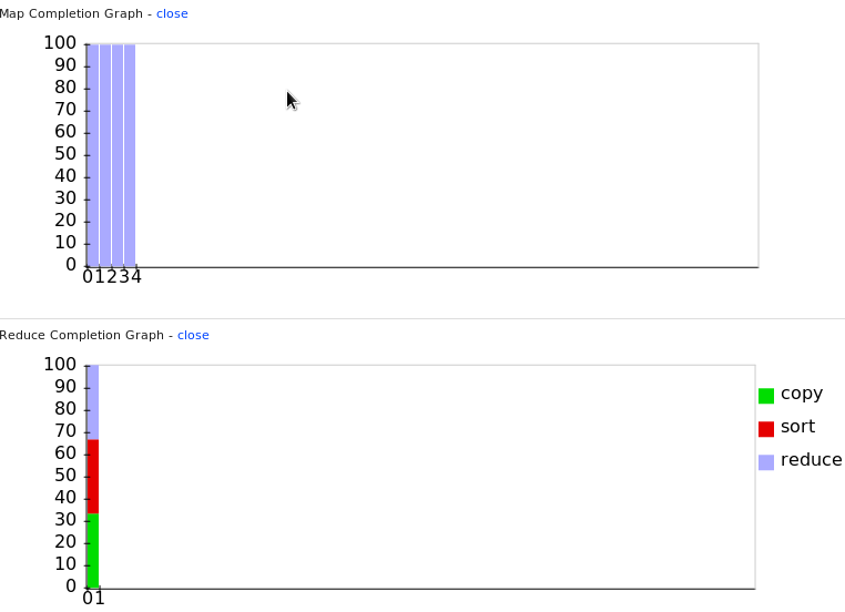
Sqoop is a handy tool to transfer bulk data between Hadoop and relational databases. It connects to MySQL via JDBC and automatically creates MapReduce functions with some simple commands. After MapReduce, the data from HDFS will be persistently and locally stored on MySQL.

# Use Sqoop to run MapReduce and export the tab delimited
# text file under specified directory to MySQL
sqoop export --username mysql-username --password mysql-pwd  \
    --export-dir myinput                    \
    --input-fields-terminated-by '\t'       \
    --input-lines-terminated-by '\n'        \
    --connect jdbc:mysql://localhost/test1  \
    --table purchases

On the client

Finally on the client installed with SAS, the PROC SQL’s pass-through mechanism will empower the user to explore or download the data stored in MySQL at the node, which will be free of any of the Hadoop’s constraints.

proc sql;    
   connect to mysql (user=mysql-username password=mysql-pwd server=mysqlserv database=test1 port=11021);
   select * from connection to mysql
       (select * from purchases limit 10000);
    disconnect from mysql;
quit;

PROC PLS and multicollinearity

Multicollinearity and its consequences

Multicollinearity usually brings significant challenges to a regression model by using either normal equation or gradient descent.

1. Invertible SSCP for normal equation

According to normal equation, the coefficients could be obtained by . If the SSCP turns to be singular and non-invertible due to multicollinearity, then the coefficients are theoretically not solvable.

2. Unstable solution for gradient descent

The gradient descent algorithm seeks to use iterative methods to minimize residual sum of squares (RSS). For example, as the plot above shows, if there is strong relationship between two regressors in a regression, many possible combinations of  and  lie along a narrow valley, which all corresponds to the minimal RSS. Thus  can be negative, positive or even zero, which becomes a confounding effect with respect to a stable model.

Partial Least Squares v.s. Principle Components Regression

The most direct way to deal with multicollinearity is to break down the regressors and construct new orthogonal variables. PLS and PCR are both dimension reduction methods that eliminate multicollinearity. The difference is that PLS also implements the response variable to select the new components. PLS is particularly useful in answering questions with multiple response variables. The PLS procedure in SAS is a powerful and flexible tool applying either PLS or PCR. One book, An Introduction to StatisticalLearning, suggests PCR over PLS.

While the supervised dimension reduction of PLS can reduce bias, it also has the potential to increase variance, so that the overall benefit of PLS relative to PCR is a wash.

In the example using the baseball data set below, with 10-fold cross-validation, PLS chooses 9 components, while PCR picks out 5.

filename myfile url 'https://svn.r-project.org/ESS/trunk/fontlock-test/baseball.sas';
%include myfile;
proc contents data=baseball   position;
   ods output position = pos;
run;

proc sql;   
   select variable into: regressors separated by ' '
   from pos
   where num between 5 and 20;
quit;
%put ®ressors;

data baseball_t;
   set baseball;
      logsalary = log10(salary);
run;

proc pls data=baseball_t censcale nfac=10 cv=split(10);
   title 'partial least squares';
   model logsalary=®ressors;
run;

proc pls data=baseball_t censcale method = pcr nfac=10 cv=split(10);
   title 'princinple components regression';
   model logsalary=®ressors;
run;

Use R in Hadoop by streaming

It seems that the combination of R and Hadoop is a must-have toolkit for people working with both statistics and large data set.

An aggregation example

The Hadoop version used here is Cloudera’s CDH4, and the underlying Linux OS is CentOS 6. The data used is a simulated sales data set form a training course by Udacity. Format of each line of the data set is: date, time, store name, item description, cost and method of payment. The six fields are separated by tab. Only two fields, store and cost, are used to aggregate the cost by each store.

A typical MapReduce job contains two R scripts: Mapper.R and reducer.R.

Mapper.R

# Use batch mode under R (don't use the path like /usr/bin/R)  
#! /usr/bin/env Rscript  

options(warn=-1)  

# We need to input tab-separated file and output tab-separated file   

input = file("stdin", "r")  
while(length(currentLine = readLines(input, n=1, warn=FALSE)) > 0) {  
   fields = unlist(strsplit(currentLine, "\t"))  
   # Make sure the line has six fields  
   if (length(fields)==6) {  
       cat(fields[3], fields[5], "\n", sep="\t")  
   }  
}  
close(input)

Reducer.R

#! /usr/bin/env Rscript  

options(warn=-1)  
salesTotal = 0  
oldKey = ""  

# Loop around the data by the formats such as key-val pair  
input = file("stdin", "r")  
while(length(currentLine = readLines(input, n=1, warn=FALSE)) > 0) {  
  data_mapped = unlist(strsplit(currentLine, "\t"))  
  if (length(data_mapped) != 2) {  
    # Something has gone wrong. However, we can do nothing.  
    continue  
  }   

  thisKey = data_mapped[1]  
  thisSale = as.double(data_mapped[2])  

  if (!identical(oldKey, "") && !identical(oldKey, thisKey)) {  
    cat(oldKey, salesTotal, "\n", sep="\t")  
    oldKey = thisKey  
    salesTotal = 0  
  }  

  oldKey = thisKey  
  salesTotal = salesTotal + thisSale  
}  

if (!identical(oldKey, "")) {  
  cat(oldKey, salesTotal, "\n", sep="\t")  
}  

close(input)

Testing

Before running MapReduce, it is better to test the codes by some linux commands.

# Make R scripts executable   
chmod w+x mapper.R  
chmod w+x reducer.R  
ls -l  

# Strip out a small file to test   
head -500 purchases.txt > test1.txt  
cat test1.txt | ./mapper.R | sort | ./reducer.R

Execution

One way is to specify all the paths and therefore start the expected MapReduce job.

hadoop jar /usr/lib/hadoop-0.20-mapreduce/contrib/streaming/hadoop-streaming-2.0.0-mr1-cdh4.1.1.jar   
-mapper mapper.R –reducer reducer.R   
–file mapper.R –file reducer.R   
-input myinput  
-output joboutput

Or we can use the alias under CDH4, which saves a lot of typing.

hs mapper.R reducer.R myinput joboutput

Overall, the MapReduce job driven by R is performed smoothly. The Hadoop JobTracker can be used to monitor or diagnose the overall process.

Rhadoop or streaming?

RHadoop is a package developed under Revolution Alytics, which allows the users to apply MapReduce job directly in R and is surely a much more popular way to integrate R and Hadoop. However, this package currently undergoes fast evolution and requires complicated dependency. As an alternative, the functionality of streaming is embedded with Hadoop, and supports all programming languages including R. If the proper installation of RHadoop poses a challenge, then streaming is a good starting point.

A cheat sheet for linear regression validation

The link of the cheat sheet is here.

I have benefited a lot from the UCLA SAS tutorial, especially the chapter of regression diagnostics. However, the content on the webpage seems to be outdated. The great thing for PROC REG is that it creates a beautiful and concise 3X3 plot panel for residual analysis.

I created a cheat sheet to try to interpret the diagnosis panel. Thanks to the ESS project, the BASEBALL data set used by SAS is available for public. Hereby I borrowed this data set as an example, and the cheat sheet also contains the data and the SAS program. The regression model attempts to predict the baseball players’ salary by their performance statistics. The plot panel can be partitioned into four functional zones:

1. OLS assumption check
   The three OLS assumption is essential to linear regression for BLUE estimators. However, the residual plot above on the left-top panel has a funnel-like shape, which is usually corrected by a log transformation in practice.
2. Normality check
   In reality the normality is not required for linear regression. However, most people like to see t-test, F-test or P value which needs the normality of residual. The histogram and Q-Q plot on the left-bottom are good reference.
3. Outlier and influential points check
   The three top-right plots can be used to rule out some extraordinary data points by leverage, Cook’s D and R-studentized residues.
4. Non-linearity check
   Rick Wicklin has a thorough introduction about the fit-mean plot. We can also look at r-square in the most bottom-right plot . If the linearity is not very satisfied, SAS/STAT has a few powerful procedures to correct non-linearity and increase the fitting performance, such as the latest ADAPTIVEREG procedure (see a diagram in my previous post).

There are still a few other concerns that need to be addressed for linear regressio such as multicolinearity (diagnosed by the VIF and other options in PROC REG) and overfitting (PROC GLMSELECT now weights in).

The PROC procedure in SAS solves the parameters by the normal equation instead of the gradient descent, which makes it always an ideal tool for linear regression diagnosis.

/*I. Grab the football data set from web */
filename myfile url 'https://svn.r-project.org/ESS/trunk/fontlock-test/baseball.sas';
%include myfile;

proc contents data=baseball   position;
   ods output position = pos;
run;

/*II. Diagnose the multiple linear regression for the players’ salaries*/
proc sql;   
   select variable into: regressors separated by ' '
   from pos
   where num between 5 and 20;
quit;
%put &regressors;

proc reg data=baseball;
   model salary = &regressors;
run;

/*III. Deal with heteroscedasticity*/
data baseball_t;
   set baseball;
   logsalary = 
      log10(salary);
run;

proc reg data=baseball_t;
   model logsalary =    
      &regressors;
run;

Kernel selection in PROC SVM

The support vector machine (SVM) is a flexible classification or regression method by using its many kernels. To apply a SVM, we possibly need to specify a kernel, a regularization parameter c and some kernel parameters like gamma. Besides the selection of regularization parameter c in my previous post, the SVM procedure and the iris flower data set are used here to discuss the kernel selection in SAS.

Exploration of the iris flower data

The iris data is classic for classification exercise. If we use the first two components from Principle Component Analysis (PCA) to compress the four predictors, petal length, petal width, sepal length, sepal width, to 2D space, then two linear boundaries seem barely able to separate the three different species such as Setosa, Versicolor and Virginica. In general, the SASHELP.IRIS is a well-separated data set for the response variable

****(1). Data exploration of iris flower data set****;
data iris;
   set sashelp.iris;
run;

proc contents data=iris position;
run;

proc princomp data=iris out=iris_pca;
   var Sepal: Petal:;
run;

proc sgplot data=iris_pca;
   scatter x = prin1 y = prin2 / group = species;
run;

PROC SVM with four different kernels

Kernel methods	Option in SAS	Formula	Parameter in SAS
linear	linear	u’*v	NA
polynomial	polynom	(gamma*u’*v + coef)^degree	K_PAR
radial basis	RBF	exp(-gamma*|u-v|^2)	K_PAR
sigmoid	sigmoid	tanh(gamma*u’*v + coef)	K_PAR; K_PAR2

PROC SVM in SAS has provided a range of kernels for selection, including ERBF, FOURIER, LINEAR, POLYNOM, RBF, RBFREC, SIGMOID and TANH. Another great thing is that it supports cross-validation including Leave-One-Out Cross-Validation ( by loo option in PROC SVM) and k-Fold Cross-Validation (by split option in PROC SVM).

Here the error rates of Leave-One-Out Cross-Validation is used to compare the performance among the four common kernels including linear, radial basis function, polynomial and sigmoid. And in this experiment most time the parameters such as c and gamma are arbitrarily set to be 1. As the result showed in the bar plot, the RBF and linear kernels bring great results, while RBF is slightly better than linear. On the contrary, the polynomial and sigmoid kernels behave very badly. In conclusion, the selection of kernel for SVM depends on the reality of the data set. A non-linear or complicated kernel is actually not necessary for an easily-classified example like the iris flower data set.

****(2). Cross validation error comparison of 4 kernels****;
proc dmdb batch data=iris dmdbcat=_cat out=_iris;
   var Sepal: Petal:;
   class species;
run;

%let knl = linear;
proc svm data=_iris dmdbcat=_cat kernel=&knl c=1 cv =loo;
   title "The kernel is &knl";
   ods output restab = &knl;
   var Sepal: Petal:;
   target species;
run;

%let knl = rbf;
proc svm data=_iris dmdbcat=_cat kernel=&knl c=1 K_PAR=1 cv=loo;
   title "The kernel is &knl";
   ods output restab = &knl;
   var Sepal: Petal:;
   target species;
run;

%let knl = polynom;
proc svm data=_iris dmdbcat=_cat kernel=&knl c=1 K_PAR =3 cv=loo;
   title "The kernel is &knl";
   ods output restab = &knl;
   var Sepal: Petal:;
   target species;
run;

%let knl = sigmoid;
proc svm data=_iris dmdbcat=_cat kernel=&knl c=1 K_PAR=1 K_PAR2=1 cv=loo;
   title "The kernel is &knl";
   ods output restab = &knl;
   var Sepal: Petal:;
   target species;
run;

data total;   
   set linear rbf polynom sigmoid;
   where label1 in ('Kernel Function','Classification Error (Loo)');
   cValue1 = lag(cValue1);
   if missing(nValue1) = 0;
run;

proc sgplot data=total;
   title " ";
   vbar cValue1 / response = nValue1;
   xaxis label = "Selection of kernel";
   yaxis label = "Classification Error by Leave-one-out Cross Validation"; 
run;

When ROC fails logistic regression for rare-event data

ROC or AUC is widely used in logistic regression or other classification methods for model comparison and feature selection, which measures the trade-off between sensitivity and specificity. The paper by Gary King warns the dangers using logistic regression for rare event and proposed a penalized likelihood estimator. In PROC LOGISTIC, the FIRTH option implements this penalty concept.

When the event in the response variable is rare, the ROC curve will be dominated by minority class and thus insensitive to the change of true positive rate, which provides litter information for model diagnosis. For example, I construct a subset of SASHELP.CARS with the response variable Type including 3 hybrid cars and 262 sedan cars, and hope to use the regressors, Weight, Wheelbase, Invoice to predict whether a car’s type is either hybrid or sedan. After the logistic regression, the AUC tents to be 0.9109 that is a pretty high value. However, the model is still ill-fitted and needs tuning, since the classification table shows the sensitivity is zero.

data rare;
    set sashelp.cars;
    where type in ("Sedan", "Hybrid");
run;

proc freq data = rare;
    tables type;
run;

proc logistic data = rare;
    model Type(event='Hybrid') = Weight Wheelbase Invoice 
       / pprob = 0.01 0.05 pevent = 0.5 0.05 ctable; 
    roc;
run;

Prob Event	Prob Level	Correct Event	Correct Non-Event	Incorrect Event	Incorrect Non-Event	Accuracy	Sensitivity	Specificity	False POS	False NEG
0.500	0.010	2	211	51	1	73.6	66.7	80.5	22.6	29.3
0.500	0.500	0	262	0	3	50.0	0.0	100.0	.	50.0
0.050	0.010	2	211	51	1	79.8	66.7	80.5	84.7	2.1
0.050	0.500	0	262	0	3	95.0	0.0	100.0	.	5.0

Solution

In case that ROC won’t help PROC LOGISTIC any more, there seem three ways that may increase the desired sensitivity or boost the ROC curve.

1. Lower the cut-off probability
   In the example above, moving the cut-off probability to an alternative value to 0.01 will significant increase the sensitivity. However, the result comes with the drastic loss of specificity as the cost.
2. Up-sampling or down-sampling
   Imbalanced classes in the response variable could be adjusted by unequal weight such as up-sampling or down-sampling. Down-sampling, would be easy to fulfill using a stratified sampling by PROC SURVEYSELECT. Up-sampling is more appropriate for this case, but may need over-sampling techniques in SAS.
3. Use different criterions such as F1 score
   For modeling rare event classification, the most important factors should be sensitivity and precision, instead of accuracy that combines sensitivity and specificity. On the contrary, the F1 score can be interpreted as a weighted average of the sensitivity and precision, which makes it a better candidate to replace AUC.
   

Some popular regression procedures in SAS/STAT

With the new release of PROC ADAPTIVEREG in SAS 9.4, the tool belt of regressions in SAS/STAT is almost completed. Hope in the future there will be a designated procedure for k-NN in SAS/STAT.

. 

The KFC toy problem: perspectives from four job roles

There is an interesting question —

There are 5 different types of toys at a KFC restaurant. If you go there, you will get one toy randomly. How many times do you need to go to KFC in order to get all 5 toys?

The question is about probabilistic analysis. Different professionals, such as a business analyst, a statistical programmer, a mathematician and a software developer, will have different thinking pathway to solve this problem. Let's see what they would think.

1. Business Analyst

A business analyst will tend to do scenario analysis at the first step.

Best-case scenario:

Assume I am so lucky that each time I visit KFC and get a different toy, then I only need 5 times to have all the five toys. The minimum number is 5.

Worst-case scenario:

To get a different toy I need to go to KFC five times. If there is not the toy I want, I will come back with empty hand. Thus, I will have to go to KFC 5*5 = 25 times. Of course, this scenario never happens.

OK. Then the mean times I need to go to KFC seems to be in a range [5, 25). Let's give the simplest try — use the (5+25)/2 to get 15 times. The number is not accurate but at least we have an estimate.

2. Statistical Programmer

As a brute-force tool, simulation is the instant thought for a statistical programmer. Let the computer randomly create 10,000 trials — say a person plays the game 10,000 times. After averaging the results, the computer eventually tells the expected times to get the 5 toys.

I modified the SAS code from a post by Rick Wicklin, and set the maximum number of visits to KFC as 32. After 10,000 runs, the mean is 11.37. The hunch tells that this number should be quite close.

************(1)Simulate 10000 trials**************************;
proc iml;
   K = 5; /* number of toys */
   L = 32; /* max visits per trial */
   /* generate NSim trials of L visits */
   NSim = 10000;
    x = j(Nsim, L);
   call randseed(12345);
   call randgen(x, "Uniform");
   x = ceil(K*x); /* integers in [1,K] */
   /* record the visit when 5 toys are taken */
   c = j(NSim,1,0); /** allocate */
    do i = 1 to NSim;
      do j = 5 to L;
         rowUnique = countunique(x[i, 1:j]);
         if rowUnique = 5 then do;
            c[i, 1] = j;
            goto skip;
         end;
      end;
      skip:
    end;
   /* output the result */
   create _1 from c;
      append from c;
   close _1;
;quit;

data _2;
   set _1;
   /* remove the trials that didn't get 5 toys in 32 visits */
   where col1 >= 5;
 run;
************(2)Show the results*******************************;
proc sgplot;
   density col1;
   density col1 / type = kernel;
run;

proc means;
run;

3. Mathematician

Actually this question is a variant of Coupon collector's problem. The mean/expectation and standard deviation can be derived directly by the formulas. The final expectation should be 5*(1+1/2+1/3+1/4+1/5) = 11.41. This is the answer.

4. Software Developer

A software developer considers time complexity and space complexity first. When N is approaching infinity, the question is similar to a merge sorting. Given a merge sort is O(nlog(n)), the expected times must be greater than 5*ln(5) = 8.05. At least this number will be a lower bound for this question.

Use MongoDB as a JSON factory

MongoDB is a persistent data store for JSON formatted data, which seems like an ideal middleware between the data tier software and the web. With MongoDB, Javascript's Map/Reduce functionality makes many trivial jobs particularly easy, such as translate an object to an array. For example, we can produce a bubble plot with Highcharts.js and the SASHEP.IRIS dataset in SAS very quickly.

Step 1: push SAS dataset toward MongoDB

First, let's push the SASHEP.IRIS dataset from SAS to MongoDB using thesas2mongo macro.

%sas2mongo(data = sashelp.iris, dbname = demo, collname = iris, tmpfolder = c:\tmp, mongofolder =c:\mongodb\bin);

Step 2: make the JSON file

Under the MongoDB shell, we could use Javascript'smap function to transform data to the desired structure.

var species = ["Setosa", "Versicolor", "Virginica"];
for (i=0; i<3; i++) {
   var z = db.iris.find({Species: species[i]}, {SepalLength:1,SepalWidth:1, PetalWidth:1, _id:0}).toArray().map(function(d){return [d.SepalLength, d.SepalWidth, d.PetalWidth]});
   print("{name:", JSON.stringify(species[i]), ", data:", JSON.stringify(z), "},");
};

Step 3: finalize Highcharts.js

The link of the final plots is here.

The plots are demonstrated into a Bootstrap 3 framework. One great advantages for SVG is that it is responsive to the devices‘ screens, which is especially friendly to mobile. The PNG or JPG formatted images can invoke Bootstrap’s responsive library to have the same effect.