Use D3.js to draw pie chart instead of PROC GCHART

Is the pie really round?

Commonly the PIE statement in the PROC GCHART produces the pie charts. Given the shortcoming of the pixel based Gxxxxxx procedures, the boundary of the pie is not very clear. I always feel that the resulting pie is not 100% round. Let's see one example with a dataset from SAS's online document.

/* Set the graphics environment */
goptions reset=all;  

/* Create the input data set SALES */
data sales;
   input site $ 1-8 count;
   datalines;
Atlanta  103
Chicago  486
Dallas   195
Denver   400
New York 307
Seattle  577
;
run;

/* Produce the chart */
proc gchart data=sales;
   pie site / sumvar=count slice = inside value = none noheading;        
run;

My intuition is that the pie above has bumps on the boundary areas. In SAS, the SVG-based SG procedures can be a rescue. However, right now they don't include an option of the PIE chart (because a pie chart is not a statistical graph?)

An alternative solution

D3.js, an already very popular open-source JavaScript library, will soon launch its 3rd version. With the JavaScript interpreter of any browser such as Chrome, IE9 or Firefox, we can make a variety of data-driven graphs with D3. The good thing is that D3 generates SVG, which can be zoomed to any size without losing detail.

In this example, I switch to a plug-in of D3 to draw the pie again. This time I finally obtain a really round pie.

Sorting in Python

#-------------------------------------------------------------------------------
# Name:        Methods of sorting
# Purpose:     implements the sortings mentioned by Robert Sedgewick and
#               Kevin Wayne, Algorithms 4ed
#
#-------------------------------------------------------------------------------

def selection_sort(a):
    for i in range(len(a)):
        min = i
        for j in range(i+1, len(a)):
            if a[j] < a[min]:
                min = j
        a[i], a[min] = a[min], a[i]

def insertion_sort(a):
    for i in range(len(a)):
        j = i
        while j > 0:
            if a[j] < a[j-1]:
                a[j], a[j-1] = a[j-1], a[j]
            j -= 1

def shell_sort(a):
    h = 1
    while h <= len(a)/3:
        h = 3*h+ 1 # in the test use 4 as increment sequence
    while h >= 1:
        for i in range(len(a)):
            j = i
            while j >= h and a[j] < a[j-h]:
                a[j], a[j-h] = a[j-h], a[j]
                j -= h
        h /= 3

def merge_sort(x):
    result = []
    if len(x) < 2:
        return x
    mid = int(len(x)/2)
    y = merge_sort(x[:mid])
    z = merge_sort(x[mid:])
    i = 0
    j = 0
    while i < len(y) and j < len(z):
        if y[i] > z[j]:
            result.append(z[j])
            j += 1
        else:
            result.append(y[i])
            i += 1
    result += y[i:]
    result += z[j:]
    return result

def quick_sort(a):
     if len(a) <= 1:
          return a
     else:
          return quick_sort([x for x in a[1:] if x < a[0]]) + [a[0]] \
                + quick_sort([x for x in a[1:] if x >= a[0]])

if __name__ == '__main__':
    a = [7, 10, 1, 1, 3, 4, 5, 9, 2, 8]
    b = {}
    for i in range(1, 6):
        b['test'+str(i)] = a[:]
    # Test the three simple sortings
    insertion_sort(b['test1'])  #1
    selection_sort(b['test2'])  #2
    shell_sort(b['test3'])      #3
    print b
    # Test the sortings that requires recursion
    print merge_sort(b['test4'])        #4
    print quick_sort(b['test5'])        #5
    # Timsort that is native in Python
    a.sort()                            #6
    print a

​

SAS and VBA (8): What VBA can do for SAS?

The eventual answer is user interface (I really don't mean SAS/AF) with or without Excel.

In the Windows environment, SAS provides data access layer by ADO and ADO.NET. We can build the applications using SAS at the backend through ADO.NET. Since Visual Basic.NET has the similar syntax to VBA, if somebody is comfortable to code in Microsoft's Visual Studio, then developing a desktop app is always feasible although it requires quite a few efforts.

For example, let's run a simple linear regression using the variable of WEIGHT to predict HEIGHT based on the SASHELP.CLASS data set. We can use Excel's macro to fetch the output by SAS as a new result sheet in the same workbook. Similarly, a desktop application (.exe) will run SAS as batch mode without notice and return the regression result in a browser. The best part of developing such an application is that Excel or Visual Studio comes at nearly no cost. And as you know, the client doesn't need to know anything about SAS.

The UI in Excel

After hitting the button

The UI of a desktop app

After hitting the button

SAS and VBA (7): calculate running total

This is a simple routine for a lot of reporting work. Many people tend to do it in Excel by dragging the range after entering the formula in the 1st cell. However, coding in VBA and SAS will usually do it in more prompt and safe way.

VBA

VBA’s unique R1C1 formula is pretty handy once we get to know the rule. The 1st cell at the F column has different R1C1 formula than the cells below.

Sub Rt()
'   Find the last row
    FinalRow = Cells(Rows.Count, 2).End(xlUp).Row
    Range("F1").Value = "Running total of Weight"
    Range("F2").FormulaR1C1 = "=RC[-1]"
    Range("F3:F" & FinalRow).FormulaR1C1 = "=RC[-1] + R[-1]C"
End Sub

SAS

It is incredibly easy to do the job in SAS. One line of code -- that is all! Obviously SAS beats VBA's three lines in this demo here.

data want;
   set sashelp.class;
   label total_weight = "Running total of Weight"; 
   total_weight + weight;
run;

SAS and VBA (6) : delete empty rows

One tricky question of the data work is to delete empty rows/observations in a raw file. A code snippet is particular useful to handle such cases. At the mean time, we need to know how many rows are actually removed as the execution result. The good news is that as programmable softwares, Excel/VBA and SAS are both good at dealing this job. In a simple demo text file below, there are actually two empty lines that have to be removed.

  
ptno visit weight
1 1 122  
1 2   
1 3   
1 4 123  
2 1 156  
2 3   

3 1 112  
3 2   

4 1 125 
4 2  
4 3 

VBA
VBA's CountA function is able to count the number of non-empty cells in any range of cells.Within a loop from the top to the bottom, it will help automatically remove those empty rows. In the codes, a message box is created to return the number of the rows deleted.

Sub DelEptRow()
    Dim myRow, Counter As Integer
    Application.ScreenUpdating = False
    For myRow = ActiveSheet.UsedRange.Rows.Count To 1 Step -1
        If Application.WorksheetFunction.CountA(Rows(myRow)) = 0 Then
            Rows(myRow).Delete
            Counter = Counter + 1
        End If
    Next myRow
    Application.ScreenUpdating = True
'   Display the number of rows that were deleted
    If Counter > 0 Then
        MsgBox Counter & " empty rows were removed"
    Else
        MsgBox "There is no empty row"
    End If
End Sub

SAS
SAS can do the same thing with the combination of its MISSING function(decides if there is any missing value) and CATS function(concatenates all numerical and string variables and trims leading blanks). It is very convenient to apply the logic in a DATA STEP and let LOG tell how many lines are deleted.

data patient;  
   input @1 ptno @3 visit @5 weight;  
   infile datalines missover;   
   cards;  
1 1 122  
1 2   
1 3   
1 4 123  
2 1 156  
2 3   

3 1 112  
3 2   

4 1 125 
4 2  
4 3 
;;;  
run;

options missing = ' ';
data want;
   set patient nobs = inobs end = eof;
   if missing(cats(of _all_)) then delete;
*  Display the number of rows that were deleted;
   outobs + 1;
   counter = inobs - outobs;
   if eof then do;
      if counter > 0 then put counter "empty rows were removed";
      else put "There is no empty row";
   end;
   drop counter outobs;
run;

Conclusion
In a DATA STEP, SAS's implicit loop has two sides. The good side is that we do not need care about how to set up a loop most time which saves codes. The bad side is that sometimes it is hard to control which row we need to loop to.

SAS and VBA (5) : replace values quickly

SAS and VBA both have their unique and quick ways to replace values in one or multiple columns.

VBA
VBA has a wonderful function Replace for several columns or regions, where the changes are likely to be happened.

Sub Replace()
   With Columns("B")
      .Replace "F", "Female"
      .Replace "M", "Male"
   End With
End Sub

SAS
User-defined format by PROC FORMAT is the best way for quick replacements.

proc format;
   value $sex
      'F' = 'Female'
      'M' = 'Male'
   ;
run;

data want;
   set sashelp.class;
   format sex $sex.;
run;

Conclusion
For some data management operations such as string/number replacement, it is better way to use the languages' built-in features, instead of the loops and condition statements.

SAS and VBA (4) : fill missing values with last valid observation

In many data management routines, it is common to fill the missing values with the last valid one. For example, we want to maintain the patient visit log about several patients, which records their weight for each visit. Given these patients’ absence for the appointments, the data analyst has to fill the the empty weight value with the last valid observation. This log includes three columns: patient ID, visit ID and weight.

ptno visit weight
1 1 122  
1 2   
1 3   
1 4 123  
2 1 156  
2 3   
3 1 112  
3 2   
4 1 125 
4 2  
4 3   

VBA 

VBA is quite flexible at those occasions. If the cell has missing value, we can assign a R1C1 formula to the cell to obtain non-missing value directly from its top neighboring cell. As the result, the logic is a simple one-sentence clause.

Sub Locf()
'  If a cell in the 3rd column is blank then fill with the previous non-missing value
   Range("C1").CurrentRegion.SpecialCells(xlCellTypeBlanks).FormulaR1C1 = "=R[-1]C"
'  Format patient ID with 000
   Columns("A").NumberFormat = "000"
End Sub

SAS

In SAS, we need to set up a temporary variable in a DATA STEP to memorize the valid value by the RETAIN statement. Then a conditional structure is used to exchange the values between the weight variable and the temporary variable.

data patient;  
   input @1 ptno @3 visit @5 weight;  
   infile datalines missover;   
   cards;  
1 1 122  
1 2   
1 3   
1 4 123  
2 1 156  
2 3   
3 1 112  
3 2   
4 1 125 
4 2  
4 3 
;;;  
run;  

data result;
   set patient;
*  Format patient ID with 000;
   format ptno z3. ; 
   retain tempvar 0;
   if missing(weight) = 1 then weight = tempvar;
   else tempvar = weight;
   drop tempvar;
run;

Conclusion
SAS is a procedural language, while VBA enjoy its power based on its many objects and properties. However, one common thing in writing good codes for both of them is to avoid the unnecessary explicit loops.

SAS and VBA (3) : lower triangle multiplication table

Flow control and looping is a very important aspect for any programming language. To see how to index a particular value in the languages’ default data type, creating a lower triangle multiplication table looks like a good test, since it is a simple question but still requires the skills to implement a nested loop and a condition statement.

VBA 

Excel has row number (1, 2, etc.) and column number (A, B, etc.) for each cell. Then in VBA, we can use Range() or Cells() to select those cells in any particular worksheet. So it will be very easy to implement the logic in VBA to create a lower triangle multiplication table.

Sub Mt()
   ActiveSheet.Range("A:Z").EntireColumn.Clear
   For i = 1 To 9
      For j = 1 To 9
         If i >= j Then
            Cells(i, j) = i*j
         End If
      Next j
   Next i
   MsgBox "Done"
End Sub

SAS 

SAS’s data set doesn’t have exact indexes for row or column. There is internal automatic variables, which is _N_, for rows. However, to specify the columns, we have to declare a temporary array. And in this demo, the position of the OUPUT statement has to be between the inner loop and the outer loop.

data mt;
   array a[9] col1-col9;   
   do i = 1 to 9;           
      do j= 1 to 9;   
         if i >= j then a[j] = i*j;   
      end;
      output;         
   end;
   drop i j;
   put "Done";
run;

Conclusion 
To select a few columns or variables, array is a must in SAS. That is possible why the DATA STEP array is so important in SAS. For beginners, VBA is an easier way to apply loops.

SAS and VBA (2) : cross tabulation and bar chart

No other tools can challenge Excel’s stance in the data analysis world. I didn’t spot many computers that are not installed with it, and I assume that everybody who faces a computer during work has to use it sometime. With the power of VBA, it is all programmable and could realize very complicated purposes without any mouse-clicking. While it is very popular to compare SAS and R, I feel that it is also meaningful to compare SAS and VBA, since these two are both well supported proprietary softwares from the great companies.

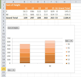
Here the example is about cross tabulation and the following visualization with a stacked bar chart. Let’s borrow the small data set SASHELP.CLASS from SAS, which includes 19 teenagers. We are interested see the total height broken down by age and sex.

Name	Sex	Age	Height	Weight
Alfred	M	14	69	112.5
Alice	F	13	56.5	84
Barbara	F	13	65.3	98
Carol	F	14	62.8	102.5
Henry	M	14	63.5	102.5
James	M	12	57.3	83
Jane	F	12	59.8	84.5
Janet	F	15	62.5	112.5
Jeffrey	M	13	62.5	84
John	M	12	59	99.5
Joyce	F	11	51.3	50.5
Judy	F	14	64.3	90
Louise	F	12	56.3	77
Mary	F	15	66.5	112
Philip	M	16	72	150
Robert	M	12	64.8	128
Ronald	M	15	67	133
Thomas	M	11	57.5	85
William	M	15	66.5	112

VBA
                                      

Pivot table has many wonderful features. It can easily aggregate data like OLAP with multiple dimensions, which makes it the most suitable tool for making cross tabs. Also because the pivot table define the fields, making a following pivot chart by codes is much more easier than any manual work.

Sub CreatePvt()
'   Set storage path for the pivot table
  Dim myPTCache As PivotCache, myPT As PivotTable
  Dim myPC As Chart

'   Delete the sheet containing the previous pivot table
  Application.ScreenUpdating = False
  On Error Resume Next
  Application.DisplayAlerts = False
  Sheets("Pivot table").Delete
  On Error GoTo 0
  
'   Create the cache
  Set myPTCache = ActiveWorkbook.PivotCaches.Create( _
      SourceType:=xlDatabase, SourceData:=Range("A1").CurrentRegion)
  
'   Add a new sheet for the pivot table
  Worksheets.Add
  ActiveSheet.Name = "Pivot table"
  
'   Create the pivot table
  Set myPT = ActiveSheet.PivotTables.Add( _
      PivotCache:=myPTCache, TableDestination:=Range("A1"))
'  Format the pivot table
   With myPT
       .AddFields RowFields:="Sex", _
           ColumnFields:="Age"
       With .PivotFields("Height")
           .Orientation = xlDataField
           ' Type of pivot table functions at http://goo.gl/F9rJh
           .Function = xlSum
           .Position = 1
        End With
       .NullString = "0"
       .DisplayFieldCaptions = False
       .TableStyle2 = "PivotStyleMedium14"
   End With
   
' Add the pivot chart
   Set ChartDataRange = myPT.TableRange1.Offset(1, 0).Resize(myPT.TableRange1.Rows.Count - 1)
   ActiveSheet.Shapes.AddChart.Select
   Set myPC = ActiveChart
' Format the pivot chart
   With myPC
       .SetSourceData Source:=ChartDataRange
      .ChartType = xlColumnStacked
      .SetElement (msoElementChartTitleAboveChart)
      .ChartTitle.Caption = " "
      .ChartStyle = 16
   End With
End Sub

SAS

In SAS, PROC REPORT is a better procedure than its older predecessors like PROC FREQ and PROC TABULATE. Similarly, the SG procedures are significantly more flexible than PROC GPLOT.

* Clear the old html outputs;
ods html close; 
ods html;

* Create the cross tabulation;
options missing = 0;
proc report data = sashelp.class nowd;
   columns sex age,height n;
   define sex / group ' ';
   define age / across ' ';
   define height / sum ' ';
   define n / 'Grand Total';
   rbreak after / summarize ;
run;
 
* Creat the statistical graph;
proc sgplot data = sashelp.class;
   vbar sex / response = height group = age;
   yaxis grid;
run;

Conclusions

In this demo, SAS would allow fewer lines of codes. Excel/VBA can do the same job and is available everywhere. And they are both highly customizable, and bring a lot fun in creating a table or a chart.

Index tuning in SAS for high-volume transactional data

Why use indexes in SAS?
A page is the smallest I/O unit that SAS can read or write, including data set page and index file page. Index files in SAS are sorting and searching structures made by B-trees. “When an index is used to process a request, such as a WHERE expression, SAS does a binary search on the index file and positions the index to the first entry that contains a qualified value. SAS then uses the value’s RID or RIDs to read the observations containing the value. The entire index file is not loaded to memory; one index page is accessed at a time. The most recent index page is kept in memory”. Thus, by scanning the index file pages first, SAS may significantly reduce the number for logical reading and physical reading, and therefore improve query performance by orders of magnitude, say from O(N) to O(log(N)) for large data set.

In this example, I simulated a data set of 10 million transaction records starting from January 1st, 2005 with 7 variables including PRIMARY_KEY, HASH_KEY, FIRST_NAME, LAST_NAME , ORDER_AMOUNT, ORDER_DATE , SHIPPING_ADDRESS. This fake transactional data set is about 600 MB big on disk.

data transaction;
   retain primary_key hash_key first_name 
      last_name order_amount order_date;
   do primary_key = 1 to 1e7;
      first_name = md5(ranuni(1));
      last_name = md5(ranuni(2));
      shipping_address = md5(ranuni(3));
      hash_key = put(md5(primary_key), hex16.);
      order_amount = put(ranuni(4)*1000, dollar8.2);
      order_date = put('01jan2005'd + floor(ranuni(5)*2500), mmddyy9.);
      output;
   end;
run;

Index strategies: 
1. Create clustered index for primary key 
Clustered index gives data the physical row order on hard disk. Not like other relational database systems, SAS doesn’t have a special statement by either PROC SQL Or Data Step, to specify a clustered index. However, I found the easiest way is to use PROC SORT to sort the data set itself.

PROC SORT is also the prerequisite of the merge join at the DATA Step, while PROC SQL mostly uses the hash join. One thing to note is that the sorting should happen before the creation of other indexes. Otherwise, after sorting the existing index files may be lost.

proc sort data = transaction;
   by primary_key;
run;

2. Create unique index for hash value 
To avoid misleading identifiers for later joining or hide sensitive information, it is quite popular nowadays to transform the primary key to the hash value for future references. SAS has a MD5 function which can generate distinguishable 128-bit hash values. To display them, I choose a valid hex16 value format.

proc sql;
   create unique index hash_key on transaction(hash_key);
quit;

3. Create simple indexes 
Individual indexes are created for each of the variables such as ORDER_DATE, ORDER_AMOUNT and SHIPPING_ADDRESS.

proc sql;
   create index order_date on transaction(order_date);
   create index order_amount on transaction(order_amount);
   create index shipping_address on transaction(shipping_address);
quit;

4. Create composite indexes 
Then another composite index is generated to include the first name and the last name, in response to full name search.

proc sql;
   create index full_name on transaction(first_name, last_name);
quit;

proc contents data = transaction position;
run;

Eventually this clustered (or sorted) data set contains 5 indexes, which are stored in a same-name index file data set that occupies 700 MB disk separately. In a conclusion, although building a few indexes for a large transactional data set is time-consuming and disk-costly, a query in PROC SQL or DATA Step by the WHERE statement is right now much faster (slash processing time up to 80%-90%), which is quite rewarding for many read-heavy jobs.

SAS and VBA (1): Conditional formatting

“Traffic lighting” applies distinctive colors to any numeric variables to indicate the ranges, which is particularly important for Excel reporting. In SAS, it can be easily realized by a user defined format. For example, if I want to add yellow color attribute to all numeric variables, which are great than 60, I can create a color format and cast it toward the target Excel file created by ODS destination.

data class;
   set sashelp.class;
run;

* Create a user defined format
proc format; 
   value range 
      60 - high = 'yellow'
      other = 'white'; 
run;

* Apply the color format for all numeric variables
ods html file = "c:\tmp\label_excel.xls" style = minimal;
proc print data = class nobs;
   var _character_ ;
   var _numeric_ / style = [background = range.];
run;
ods html close;

Similarly, a VBA subroutine can do the global search based on the specified ranges with a looping structure around the numeric variables. The looking of the resulting Excel files by either SAS or VBA are essentially identical.

Sub global_label()
    Dim Cell As Object
    Dim myCell As Range
    Dim myRange As Range
   
'   Specify selection ranges
    If TypeName(Selection) <> "Range" Then Exit Sub
    If Selection.CountLarge = 1 Then
       Set myRange = ActiveSheet.UsedRange
    Else
       Set myRange = Application.Intersect(Selection, ActiveSheet.UsedRange)
    End If
    
'   Only search numeric cells 
    On Error Resume Next
    Set myRange = myRange.SpecialCells(xlConstants, xlNumbers)
    If myRange Is Nothing Then Exit Sub
    On Error GoTo 0
    
'   Aggregate cells
    For Each Cell In myRange
        If Cell.Value > 60 Then
            If myCell Is Nothing Then
                Set myCell = Cell
            Else
                Set myCell = Application.Union(myCell, Cell)
            End If
        End If
    Next Cell

'   Label qualified cells
    If myCell Is Nothing Then
        MsgBox "No matching cell is found"
    Else
        myCell.Select
        With Selection.Interior
            .Pattern = xlSolid
            .Color = 65535
        End With
    End If
End Sub

Use the set operator UNION in PROC SQL

SQL syntax contains a few set operators, such as UNION, EXCEPT and INTERSECT. The UNION operator concatenates the results of multiple SQL queries vertically into a single table for all matching rows, which I found particularly useful in PROC SQL while using SAS to manage data. Here come two examples.

Example 1 – Transpose data
PROC SQL can transform a dataset to any desired structure, without referring to DATA step or PROC TRANSPOSE. For example, SASHELP.CLASS can be transposed from wide to long by the UNION ALL clause, and reversely from long to wide by the MAX function and the GROUP clause.

From wide to long

data wide;
   set sashelp.class;
   drop sex;
run;

proc sql;
   create table long as
   select name, 'Age' as var, age as col1
   from wide
   union all
   select name, 'Weight' as var, weight as col1
   from wide
   union all
   select name, 'Height' as var, height as col1
   from wide
;quit;

From long to wide

proc sql;
   create table wide as
   select name,
      max(case when var = 'Age' then col1 end) as Age,
      max(case when var = 'Weight' then col1 end) as Weight,
      max(case when var = 'Height' then col1 end) as Height
   from long
   group by name;
quit;

Example 2 – Aggregate data into a cube
In SAS, PROC SQL doesn’t support the ROLLUP or CUBE clause. However, we can apply multiple UNION operators to simulate such functionality. For example, we can create a cube table to list all possible summations of the ACTUAL variable by STATE, PRODUCT, YEAR in the SASHELP.PRDSAL2 dataset. Afterward we can easily query this multi-dimensional data structure to look for interesting aggregation information, without running any other aggregating procedure again.

data prdsal2;
   set sashelp.prdsal2;
run;

proc sql;
   create table cube as
   select state,product, year, 'total by state, prodcut and year' as category,
   sum(actual) as actual
   from prdsal2
   group by state, product, year
   union
   select state, product, ., 'total by state and prodcuct', sum(actual)
   from prdsal2
   group by state, product
   union
   select state,'', year, 'total by state and year', sum(actual)
   from prdsal2
   group by state, year
   union
   select '',product, year, 'total by product and year', sum(actual)
   from prdsal2
   group by product, year
   union 
   select '' ,'', year, 'total by year', sum(actual)
   from prdsal2
   group by year
   union 
   select state, '',. , 'total by state', sum(actual)
   from prdsal2   
   group by state
   union 
   select '',  product, ., 'total by product', sum(actual)
   from prdsal2
   union
   select '', '', ., 'grand total', sum(actual)
   from prdsal2
   order by state, product, year
;quit;

Transform a SAS data set to an Excel pivot table by VBA

Pivot Table in Excel is the popular data report format, which is similar to an OLAP cube that aggregates data at any dimensions. To create a pivot table for a table with lots of columns, it usually takes 100+ drags and clicks to get job done, which is somehow annoying.

I didn't try the SAS’s Add-in for Microsoft Office or SAS Enterprise Guide yet. However, an easy solution to transform a SAS data set toward an Excel pivot table is possibly to use some VBA scripts under Excel. For example, SASHELP.PRDSAL2, which is a free data set shipped with SAS, records the furniture sales in 64 states of the three countries from 1995 to 1998, and has total 23,040 observations and 11 variables. This data set can be transformed to an Excel pivot table very quickly by two simple steps.

Step 1

In SAS, a data set can be exported toward an XLS file through ODS destination. Although it is still based on HTLM format, it can be opened by Excel.

ods html file = 'c:\tmp\prdsal2.xls' style = minimal;
title;
proc print data = sashelp.prdsal2 noobs;
run;
ods html close;

Step 2

Next step we click on this file, press ALT + F11 to enter VBA editor, paste the VBA code below and run it. Then the pivot table is created. The good thing about this method is that the pivot table can be replicated anywhere by such a VBA subroutine, and it is customizable for particular needs. The example was finished in Excel 2007.

Sub createPT()
'   Set storage path for the pivot table 
    myDataset = "sashelp.prdsal2"
    myFilepath = "c:\tmp\" & myDataset & "_" & Format(Date, "dd-mm-yyyy") & ".xlsx"
    Dim myPTCache As PivotCache
    Dim myPT As PivotTable

'   Delete the sheet containing the previous pivot table   
    Application.ScreenUpdating = False
    On Error Resume Next
    Application.DisplayAlerts = False
    Sheets("Pivot_Table_Sheet").Delete
    On Error GoTo 0
    
'   Create the cache
    Set myPTCache = ActiveWorkbook.PivotCaches.Create( _
        SourceType:=xlDatabase, SourceData:=Range("A1").CurrentRegion)
    
'   Add a new sheet for the pivot table
    Worksheets.Add
    ActiveSheet.Name = "Pivot_Table_Sheet"
    
'   Create the pivot table
    Set myPT = ActiveSheet.PivotTables.Add( _
        PivotCache:=myPTCache, TableDestination:=Range("A5"))
    With myPT
        .PivotFields("COUNTRY").Orientation = xlPageField
        .PivotFields("STATE").Orientation = xlRowField
        .PivotFields("PRODTYPE").Orientation = xlRowField
        .PivotFields("PRODUCT").Orientation = xlRowField
        .PivotFields("YEAR").Orientation = xlColumnField
        .PivotFields("QUARTER").Orientation = xlColumnField
        .PivotFields("MONTH").Orientation = xlColumnField
        .PivotFields("ACTUAL").Orientation = xlDataField
        .PivotFields("PREDICT").Orientation = xlDataField
        .DataPivotField.Orientation = xlRowField
        '  Add a calculated field to compare the predicted value and the actual value
        .CalculatedFields.Add "DIFF", "=PREDICT-ACTUAL"
        .PivotFields("DIFF").Orientation = xlDataField
        ' Specify a number format
        .DataBodyRange.NumberFormat = "$#, ##0.00"
        ' Apply a style for pivot table
        .TableStyle2 = "PivotStyleLight18"
    End With
    Range("A1").FormulaR1C1 = "Pivot table made from data set" & " " & myDataset
    Range("A2").FormulaR1C1 = "Prepared by WWW.SASANALYSIS.COM on " & Date
    ActiveWorkbook.SaveAs Filename:=myFilepath, _
        FileFormat:=xlOpenXMLWorkbook, CreateBackup:=False
End Sub

Top 10 tips and tricks about PROC SQL

INTRODUCTION

PROC SQL is the implementation of the SQL syntax in SAS. It first appeared in SAS 6.0, and since then has been very popular for SAS users. SAS ships with a few sample data sets in its HELP library, and SASHELP.CLASS is one of them. This dataset contains 5 variables including name, weight, height, sex and age for 19 simulated teenagers, and in this paper I primarily use it for the demonstration purpose. Here I summarize the 10 interesting tricks and tips using PROC SQL. At the beginning, I first make a copy of SASHELP.CLASS at the WORK library and transform the row number of the data set to a new variable obs.

dataclass;

   setsashelp.class;

   /* Give an index for each child*/

   obs = _n_;

run;

1. Calculate the median of a variable

With the aggregating HAVING clause and some self-join techniques, PROC SQL can easily calculate the median for a variable.

procsql;

   selectavg(weight) as Median

   from(select e.weight

   fromclass e, class d

   groupby e.weight

   havingsum(case when e.weight = d.weight then 1else 0end)

      >= abs(sum(sign(e.weight - d.weight))));

quit;

2. Draw a horizontal histogram

A histogram visualizes the distribution pattern of a variable. PROC SQL can draw a horizontal histogram by showing the frequency bars with a few asterisks for each level of the variable age.

procsql;

   selectage, repeat('*',count(*)*4) as Frequency

   fromclass

   groupby age

   orderby age;

quit;

3. Return the running total for a variable

A running total is the summation of a sequence of numbers which is updated each time with the increase of the observations. In the example below, I calculate the running total and save them as a new variable Running_total by the SUM function and a conditional statement, which logically is similar to an example in SAS/IML[1]. 

procsql;

   selectname, weight,

      (selectsum(a.weight) from class as

      a wherea.obs <= b.obs) as Running_total

   fromclass as b;

quit;

4. Report the total number for a variable

PROC SQL is a flexible way to find the total number for any variable by its set operator UNION and the SUM function. In the example, the total number of the variable weight is reported at the bottom of the output table.

procsql;

   selectname, weight

   fromclass

   unionall

   select'Total', sum(weight)

   fromclass;

quit;

5. Retrieve the metadata for a data set

SAS stores the metadata at its DICTIONARY data sets. PROC SQL can visit the directory, retrieve the column detail, and return the information to the users.

procsql;

   selectname, type, varnum

   fromsashelp.vcolumn

   wherelibname = 'WORK' andmemname = 'CLASS';

quit;

6. Rank a variable 

Besides the designated ranking procedure PROC RANK in SAS, PROC SQL can also do some simple ranking as well.

procsql;

   selectname, a.weight, (select count(distinctb.weight)

   fromclass b

   /* Rank by the ascending order for the weight variable*/

   whereb.weight <= a.weight) as rank

   fromclass a;

quit;

7. Simple random sampling 

PROC SQL is widely used in simple random sampling. For example, I randomly choose 8 observations by the OUTOBS option at the PROC statement. The randomization process is realized by the RANUNI function at the ORDER BY statement with a seed 1234.

procsql outobs = 8;

   select*

   fromclass

   orderby ranuni(1234);

quit;

8. Replicate a data set without data

In PROC SQL, it is a fairly straightforward one-line statement to create a new empty data set while keeps all the structure of the original data set.

procsql;

   createtable class2 likeclass;

quit;

9. Transpose data

Usually DATA step ARRAY and PROC TRANSPOSE allow SAS users to restructure the data set, while PROC SQL sometimes is an alternative solution. For instance, if we need a wide-to-long operation to list the names of the children by their gender in the CLASS date set, then PROC SQL can fulfill the functionality through the combinations of some queries and subqueries.

procsql;

   selectmax(case when sex='F'

      thenname else ' ' end) as Female,

      max(casewhen sex='M'

      thenname else ' ' end) as Male

   from(select e.sex,

      e.name,

      (selectcount(*) from class d

      wheree.sex=d.sex and e.obs < d.obs) aslevel

      fromclass e)

   groupby level;

quit;

10. Count the missing values

Another advantage of PROC SQL is that its NMISS function works for both numeric and character variables [2], which makes PROC SQL an ideal tool for missing value detection.

procsql;

   selectcount(*) 'Total', nmiss(weight)

      'Number of missing values for weight'

   fromclass;

quit;

CONCLUSION

The combination of SAS’s powerful functions and the SQL procedure will benefit SAS users in data management and descriptive statistics.